Mamezou Engineering Solutions Division, Takahiro Ishii

At Mamezou, we develop various robotic technologies. Although we often develop applied technologies that meet client demands using robots from other companies, we are also developing industrial robots with 6-axis or 7-axis arms, known as robot arms or manipulators, from scratch. Through this development, we have generated various applied technologies and proposals. I would like to share the insights gained here with the readers. In this explanation, I would like to explain various mechanisms for controlling a 6-axis industrial vertical multi-joint manipulator.

This time, I will introduce an example of the detailed trajectory generation process algorithm that I explained last time. Specifically, I will discuss how to interpolate the characteristic positions and postures specified by the user to calculate samples of trajectories (sets of positions and postures).

In robot programming, the positions and postures of the tool tip that the trajectory passes through are continuously specified. Furthermore, the shape of the trajectory and the speed and acceleration between the Key Points (KPs) are also specified. These are used to sample positions and postures to form trajectory $T_i$.

Here, KPs are similarly expressed using the previously mentioned definitions of tool tip positions and postures. Here, the sequence number of the trajectory on the KP is denoted by $j$ ($j$ is a non-negative integer).

$$T_{KP[j]}=\left( \begin{array}{cccc} u_x & v_x & w_x & q_x \\ u_y & v_y & w_y & q_y \\ u_z & v_z & w_z & q_z \\ 0 & 0 & 0 & 1 \\ \end{array} \right)$$

To explain this again, the upper left 3x3 submatrix $R_{KP[j]}$ (orthonormal system) represents the posture/direction of the tool tip coordinate system from the base coordinate system $\Sigma_0$. The fourth column represents the origin position. Thus, the direction of the three axes XYZ of the tool tip coordinate system at the $j$-th is

$$\begin{align*} & \vec{X_j} = ( u_x,u_y,u_z ) \\ & \vec{Y_j} = ( v_x,v_y,v_z ) \\ & \vec{Z_j} = ( w_x,w_y,w_z ) \\ & |\vec{X_j}| = |\vec{Y_j}| =|\vec{Z_j}| =1 \\ & \vec{X_j} \cdot \vec{Y_j} =\vec{Y_j} \cdot \vec{Z_j} = \vec{Z_j} \cdot \vec{X_j}=0 \\ \end{align*}$$

and the position is

$$\vec{P}_{KP[j]} = ( q_x,q_y,q_z )$$

It is possible to determine $T_{KP[j]}$ using forward kinematics from the 6-axis joint angle vector $\Theta_j$ if necessary. Additionally, the posture $R_{KP[j]}$ can also be determined from Euler angles.

Once the trajectory between KPs is determined and the distance is set, the trapezoidal velocity profile previously explained can be determined using the velocity and acceleration.

The following explains the method of trajectory generation for each shape. The actual process is complex, so here I will limit myself to explaining the concept without delving into specific processing methods.

Consider connecting KPs in three dimensions with a straight line as described above.

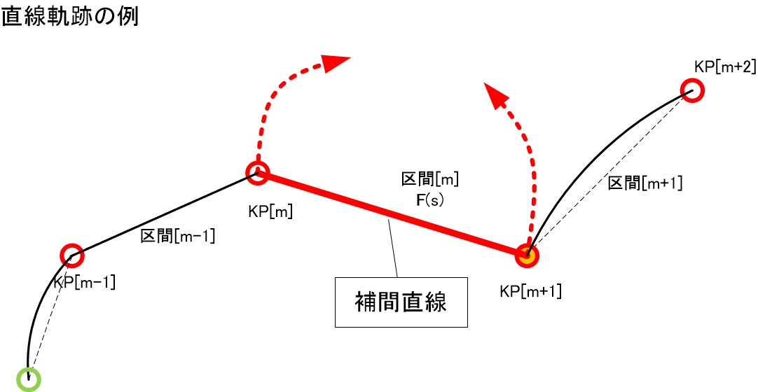
Regarding the interval number $m$ ($m$ is a non-negative integer) from KP$_{[m]}$ to KP$_{[m+1]}$, let the parameter be $s$ (>0.0) then

$$\vec{F}(s) = (1-(s-m))*\vec{P}_{KP[m]} + (s-m)*\vec{P}_{KP[m+1]}$$

$$m= \rm{floor}(s)$$

This is the formula for linear interpolation. By sampling, i.e., dividing $s$ appropriately and calculating $\vec{F}(s)$, the position trajectory can be determined. Note that at KP$_{[m]}$ (when $s=m$), the position matches, so this trajectory passes through KP.

If three or more KPs, or in other words, two or more continuous intervals are specified, a smooth three-dimensional position trajectory can be obtained through piecewise cubic spline interpolation.

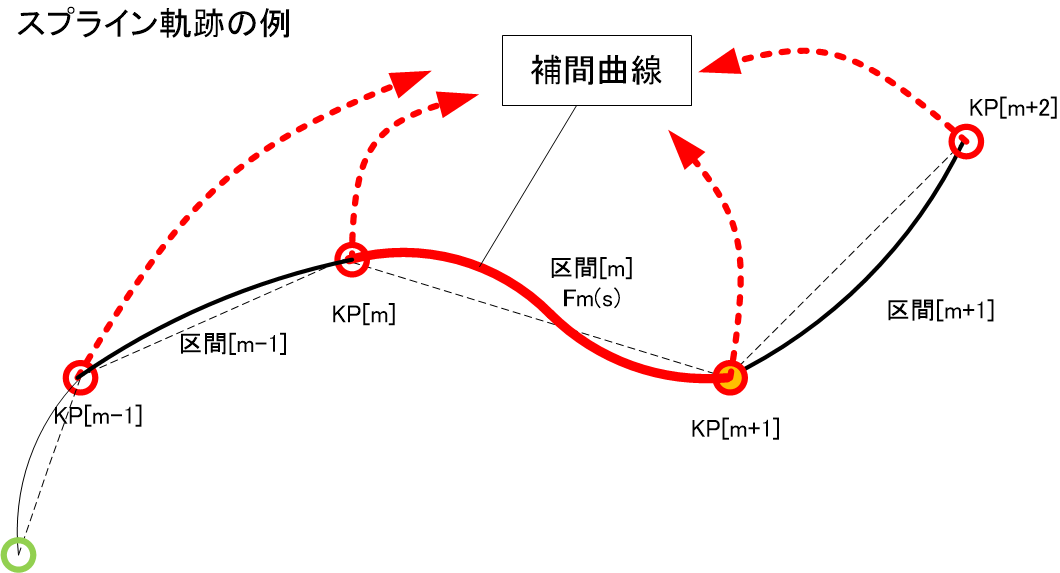
First, for interval $m$, define the piecewise cubic spline interpolation formula with the parameter $s$ as follows.

$$\vec{F}_m(s) = \vec{a}_m + \vec{b}_m*(s-m) + \vec{c}_m*(s-m)^2 + \vec{d}_m*(s-m)^3$$

This is done by setting up simultaneous equations for any $m$ such that the following conditions are met, with coefficients $\vec{a}_m, \vec{b}_m, \vec{c}_m, \vec{d}_m$ as unknowns. This solution can be performed with a unique calculation.

1. Zeroth-order continuity:

   $$\vec{P}_{KP[m]}=\vec{F_m}(m);~ \vec{P}_{KP[m+1]}=\vec{F_m}(m+1);~...$$

2. First-order continuity: Continuity of the slope of the tangent at KP

   $$\frac{d\vec{F}_{m-1}(m)}{ds}=\frac{d\vec{F}_{m}(m)}{ds};~ \frac{d\vec{F}_m(m+1)}{ds}=\frac{d\vec{F}_{m+1}(m+1)}{ds} ;~...$$

3. Second-order continuity: Continuity of curvature at KP

   $$\frac{d^2\vec{F}_{m-1}(m)}{ds^2}=\frac{d^2\vec{F}_{m}(m)}{ds^2};~ \frac{d^2\vec{F}_m(m+1)}{ds^2}=\frac{d^2\vec{F}_{m+1}(m+1)}{ds^2};~...$$

4. The slope of the tangent at the starting and ending KPs is undefined, and the curvature is set to zero.

Using the coefficients obtained in this way, $\vec{F}_m(s)$ is determined, and by sampling $s$, a sequence of sample points as a trajectory can be calculated. In this case,

$$m=\rm{floor}(s)$$

is set. This trajectory is a smooth three-dimensional curve that penetrates KP.

If two continuous intervals are specified for three KPs, a smooth three-dimensional arc trajectory can be obtained. The center and radius of the circle passing through the three points are determined, and the arc trajectory is calculated by sampling the movement angle from the center.

In fact, it is difficult to process this calculation straightforwardly in three-dimensional space, so consider it by projecting it into two dimensions first. In the figure below, the UV coordinate system is arranged with KP$_{[m]}$ as the origin, KP$_{[m-1]}$ on the U-axis, and KP$_{[m+1]}$ on the UV plane.

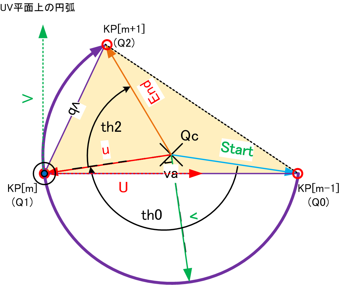
Formulating this results in the following.

$$\vec{v}_a=\vec{P}_{KP[m-1]}-\vec{P}_{KP[m]}$$

$$\vec{v}_b=\vec{P}_{KP[m+1]}-\vec{P}_{KP[m]}$$

$$\vec{U}=\vec{v}_a/|\vec{v}_a|$$

$$\vec{W}=\frac{\vec{v}_a \times \vec{v}_b}{|\vec{v}_a||\vec{v}_b|}$$

$$\vec{V}=\vec{W} \times \vec{U}$$

This allows the calculation of the 4x4 homogeneous matrix $T^{WC}_{UV}$ for converting from the UVW coordinate system to the base coordinate system $\Sigma_0$. That is, $\vec{U},\vec{V},\vec{W}$ are substituted into the rotation matrix part of the matrix, and $\vec{P}_{KP[m]}$ is substituted into the parallel translation part.

Furthermore, the angle formed by $\vec{v}_a$ and $\vec{v}_b$ can be calculated using the inner product formula, and the two-dimensional coordinates $Q_0,Q_1,Q_2$ of the three KPs on the UV coordinate system can be obtained. Then, the radius $R$ and center coordinates $Q_c(U_c, V_c)$ of the circle passing through these three points can be analytically derived in the UV coordinate system. Similarly, the rotational movement angles $th_0$ and $th_2$ around $Q_c$ can also be calculated.
Here, as shown in the figure, define the uv coordinate system with $Q_c$ as the origin and the u-axis in the direction of $Q_1$. On the UVW coordinate system, the u-axis, v-axis, and w-axis are respectively

$$\begin{align*} & \vec{u}= (-U_c/R, -V_c/R,0 ) \\ & \vec{v}= ( V_c/R, -U_c/R,0) \\ & \vec{w}= (0,0,1) \end{align*}$$

This allows the calculation of the homogeneous transformation matrix $T^{UV}_{uv}$ for converting from the uvw coordinate system to the UVW coordinate system.

From the above, the homogeneous transformation matrix $T^{WC}_{uv}$ from the uvw coordinate system to the base coordinate system $\Sigma_0$ is

$$T^{WC}_{uv} = T^{WC}_{UV} T^{UV}_{uv}$$

which can be calculated.

Now, the parametric representation of the arc from $Q_0$ in the uvw coordinate system is

$$\left( \begin{array}{ccc} u \\ v \\ w \end{array} \right) =　\left( \begin{array}{ccc} R~ \rm{cos}(-\theta) \\ R~ \rm{sin}(-\theta)\\ 0 \end{array} \right)$$

Therefore, by sampling θ from $-th_0$ to $th_2$ in sequence and using $T^{WC}_{uv}$ for coordinate transformation, a sequence of sample points of the arc in three dimensions can be calculated.

So far, I have explained the method of deriving or interpolating trajectories for the intuitively understandable tool tip "position". In contrast, "posture" also needs to be interpolated continuously between KPs and is important sample information that makes up the trajectory. "Posture" refers to the upper left 3x3 rotation matrix part of the 4x4 homogeneous matrix representing the state of the tool tip, which consists of nine numerical values as already explained. Interpolating these nine numerical values while maintaining an orthonormal system is difficult. Therefore, traditionally, these nine numerical values were once converted into a vector representing three angles, i.e., Euler angles, and the angle vectors were appropriately interpolated. However, this method did not result in natural interpolation due to the anisotropy of the three angles and did not allow efficient posture movement. Also, handling gimbal lock was difficult.

Therefore, in recent years, it has become common to represent the posture and its rotational operation in three-dimensional space set at KP using Quaternion $\bold{q}$ (Quaternion) and to perform interpolation processing between them. Note that a unit Quaternion of length 1 is used to represent rotation.

The procedure for interpolation processing is as follows.

1. Convert the rotation matrices $R$[m],$R$[m+1],... representing the postures at KP[m],KP[m+1],... belonging to the interpolated interval m into Quaternion $\bold{q}_{[m]}$, $\bold{q}_{[m+1]}$, ...
2. Interpolate between $\bold{q}_{[m]}$, $\bold{q}_{[m+1]}$, ... to smoothly generate sample $\bold{q}_{[m]}(s_i)$
3. Sequentially reverse transform $\bold{q}_{[m]}(s_i)$ into $R_{[m]}(s_i)$

For reference, the following shows an example of code for converting from $R$ to $\bold{q}$ in the above 1.

///////////////////////////////////////////////////////////
/// @brief		Set Quaternion by calculating from matrix (3x3)
/// @param[in]	_matrix
/// @return		None
/// @note
///////////////////////////////////////////////////////////
void Quaternion::SetR3x3(const Matrix& _matrix)
{
	const double m11=_matrix.At(0, 0), m12=_matrix.At(0, 1), m13=_matrix.At(0, 2);
	const double m21=_matrix.At(1, 0), m22=_matrix.At(1, 1), m23=_matrix.At(1, 2);
	const double m31=_matrix.At(2, 0), m32=_matrix.At(2, 1), m33=_matrix.At(2, 2);

	// Search for the largest component of w ( =q1 )
	double q[4]; // Candidates for w 0:w, 1:x, 2:y, 3:z
	q[0] =  m11 + m22 + m33 + 1.0;
	q[1] =  m11 - m22 - m33 + 1.0;
	q[2] = -m11 + m22 - m33 + 1.0;
	q[3] = -m11 - m22 + m33 + 1.0;

	int imax = 0;
	for ( int i=1; i<4; i++ ) {
		if ( q[i] > q[imax] ) imax = i;
	}
	if( q[imax] < 0.0 ){
		assert(0);
		m_quat1 = 1.0; m_quat2 = 0.0; m_quat3 = 0.0; m_quat4 = 0.0;
		return;
	}
	// Calculate the value of the largest element
	const double v = sqrt( q[imax] )*0.5;
	q[imax] = v;
	const double kc = 0.25/v;
	switch ( imax ) {
	case 0: // w
		q[1] = (m32 - m23) * kc;
		q[2] = (m13 - m31) * kc;
		q[3] = (m21 - m12) * kc;
		break;
	case 1: // x
		q[0] = (m32 - m23) * kc;
		q[2] = (m21 + m12) * kc;
		q[3] = (m13 + m31) * kc;
		break;
	case 2: // y
		q[0] = (m13 - m31) * kc;
		q[1] = (m21 + m12) * kc;
		q[3] = (m32 + m23) * kc;
		break;
	case 3: // z
		q[0] = (m21 - m12) * kc;
		q[1] = (m13 + m31) * kc;
		q[2] = (m32 + m23) * kc;
		break;
	}
	m_quat1 = q[0];
	m_quat2 = q[1];
	m_quat3 = q[2];
	m_quat4 = q[3];
}

Also, the following shows an example of code for reverse transformation in the above 3.

///////////////////////////////////////////////////////////
/// @brief		Calculate and output rotation matrix (3x3) from Quaternion
/// @param[out]	_matrix
/// @return		None
/// @note
///////////////////////////////////////////////////////////
void Quaternion::GetR3x3(Matrix& _matrix) const
{
	assert(_matrix.GetRow() >= 3);
	assert(_matrix.GetCol() >= 3);

	const double qw = m_quat1;
	const double qx = m_quat2;
	const double qy = m_quat3;
	const double qz = m_quat4;

	double qxy = 2.0*qx*qy;
	double qyz = 2.0*qy*qz;
	double qxz = 2.0*qx*qz;

	double qwx = 2.0*qw*qx;
	double qwy = 2.0*qw*qy;
	double qwz = 2.0*qw*qz;

	double qxx = 2.0*qx*qx;
	double qyy = 2.0*qy*qy;
	double qzz = 2.0*qz*qz;

	double &m11=_matrix.At(0, 0), &m12=_matrix.At(0, 1), &m13=_matrix.At(0, 2);
	double &m21=_matrix.At(1, 0), &m22=_matrix,.At(1, 1), &m23=_matrix.At(1, 2);
	double &m31=_matrix.At(2, 0), &m32=_matrix.At(2, 1), &m33=_matrix.At(2, 2);

	m11 = 1.0 - qyy - qzz;
	m21 = qxy + qwz;
	m31 = qxz - qwy;

	m12 = qxy - qwz;
	m22 = 1.0 - qxx - qzz;
	m32 = qyz + qwx;

	m13 = qxz + qwy;
	m23 = qyz - qwx;
	m33 = 1.0 - qxx - qyy;
}

Spherical linear interpolation (Slerp) interpolates between one posture $\bold{q}_{[m]}$ and $\bold{q}_{[m+1]}$ while moving in the shortest rotation. Imagine tracing a curve along the great circle on the surface of a 4-dimensional unit sphere between two $\bold{q}$ points placed on the sphere's surface. During this, the parameter $s$ proportionally divides the preceding and following $\bold{q}$ based on the rotation amount.

Specifically, the Quaternion $\bold{q}_{[m]}(s)$ in interval $m$ is obtained by the following procedure.

First, calculate the angle $\theta$ formed between Quaternions ("$\cdot$" denotes the dot product)

$$\theta = \rm{cos}^{-1}(\bold{q}_{[m]} \cdot \bold{q}_{[m+1]}) \\$$

Next, for parameter $s$ $(m\le s \le m+1)$, obtain the weight

$$r(s)=s-m \\$$

In this case, if $\theta \le \frac{\pi}{2}$, then

$$\begin{align*} &k_s(s)=\rm{sin}((1-r(s)) ~ \theta)/\rm{sin}(\theta) \\ &k_e(s)=\rm{sin}(\theta~ r(s))/\rm{sin}(\theta) \\ &\bold{q}_{[m]}(s)=k_s(s)~\bold{q}_{[m]} + k_e(s)~\bold{q}_{[m+1]} \\ \end{align*}$$

Otherwise, if $\theta \gt \frac{\pi}{2}$, using the antipodal equivalence of Quaternion,

$$\begin{align*} &\theta' = \pi-\theta\\ &k_s(s)=\rm{sin}((1-r(s)) ~ \theta')/\rm{sin}(\theta') \\ &k_e(s)=\rm{sin}(\theta' ~ r(s))/\rm{sin}(\theta') \\ &\bold{q}_{[m]}(s)=k_s(s)~\bold{q}_{[m]} - k_e(s)~\bold{q}_{[m+1]} \\ \end{align*}$$

is calculated.
Part of this process can be organized and defined as a function, as shown below.
That is, the Quaternion $\bold{q}$ for linear change from $\bold{q}_0$ to $\bold{q}_1$ with the interpolation ratio $r$ is calculated using the $\rm{Slerp}$ function.

$$\bold{q} =\rm{\rm{Slerp}}(r, \bold{q}_0,\bold{q}_{1} ) \\ ~ (0 \le r \le 1)$$

This section discusses methods for modifying trajectories so that both position and posture change smoothly near the boundaries of intervals. In this case, the modified trajectory no longer needs to accurately trace the position/posture of KPs placed at the boundaries.

Consider a case where a straight line trajectory is specified for one interval and an arc trajectory for the next interval. To ensure smooth operation of the tool tip, it is necessary to reduce the speed to zero at the KP placed at the boundary between the two intervals, appropriately decelerate before that, and accelerate after that. This way, even if the trajectory bends at the KP (i.e., first-order discontinuity and second-order discontinuity), stopping momentarily does not strain the joint axes. However, if you want to pass through the KP area at high speed without stopping, it is better to keep the tool tip speed as constant as possible and move without stopping. For this, it is necessary to smoothly connect the trajectories before and after the KP. This applies not only to position trajectories but also to posture trajectories.

Fitting Position Trajectories

One method is to first draw the trajectory curves specified for the previous and next intervals and then fit an appropriate curve to connect them smoothly. For example, consider the case where KP$_{[m]}$ is the interval boundary, draw the trajectory curves for intervals m-1 and m once, and consider subpoints KP$_{[m]1}$ and KP$_{[m]2}$ at appropriate distances ($L_1$, $L_2$) from KP$_{[m]}$. Let the positions at each point be $\vec{Q}_1$, $\vec{Q}_2$, and the tangent vectors be $\vec{V}_{q1}$, $\vec{V}_{q2}$. Using these, the cubic spline interpolation formula $\vec{F}_0(s) ~~ (s=0～1)$ is sampled to form a smooth curve.

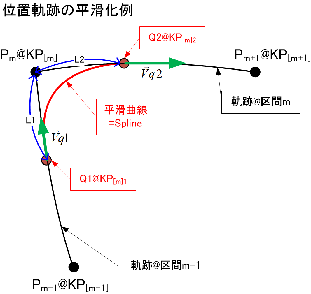
The method for obtaining this curve or interpolation formula is similar to the previously mentioned method for spline curves. However, there is only one segment, and the boundary conditions are different. They are as follows.

First, restate the cubic spline interpolation formula $\vec{F}_0(s)$.

$$\vec{F_0}(s) = \vec{a}_0 + \vec{b}_0*s + \vec{c}_0*s^2 + \vec{d}_0*s^3$$

Set up simultaneous equations such that the following conditions are met, and solve the equations with coefficients $\vec{a}_0, \vec{b}_0, \vec{c}_0, \vec{d}_0$ as unknowns. This solution can also be performed with a unique calculation.

1. Zeroth-order continuity:

   $$\vec{Q}_1=\vec{F_0}(0);~ \vec{Q}_{2}=\vec{F_0}(1)$$

2. First-order continuity: Continuity of the slope of the tangent at KP

   $$\vec{V}_{q1}=\frac{d\vec{F}_0(0)}{ds};~ \vec{V}_{q2}=\frac{d\vec{F}_0(1)}{ds}$$

In summary,

1. From KP$_{[m-1]}$ to KP$_{[m]1}$, use the original trajectory of interval m-1,
2. From KP$_{[m]1}$ to KP$_{[m]2}$, use the above spline curve,
3. From KP$_{[m]2}$ to KP$_{[m+1]}$, use the original trajectory of interval m

This results in a continuously smooth trajectory. The distances $L_1$ and $L_2$ from the KP to be smoothed can be adjusted to modify the smoothness. In this case, it is also necessary to modify the velocity profile (specifically, the norm of the velocity vector profile). After laying out the two velocity profiles for the original two intervals, the section from KP$_{[m]1}$ to KP$_{[m]2}$ is modified to:

1. Move at a constant speed as much as possible.
2. Move precisely the distance of the spline curve.

Note that distance corresponds to the integral of the velocity profile, i.e., the area of the interval.

By the way, this method requires two trajectory data for smoothing one location at the beginning of the calculation, but eventually, part of it becomes unnecessary. Be aware of the computational load and memory burden during implementation.

Fitting Posture

A method for smoothing part of the posture trajectory so that the posture trajectories before and after change smoothly throughout. For example, the following method can be used.

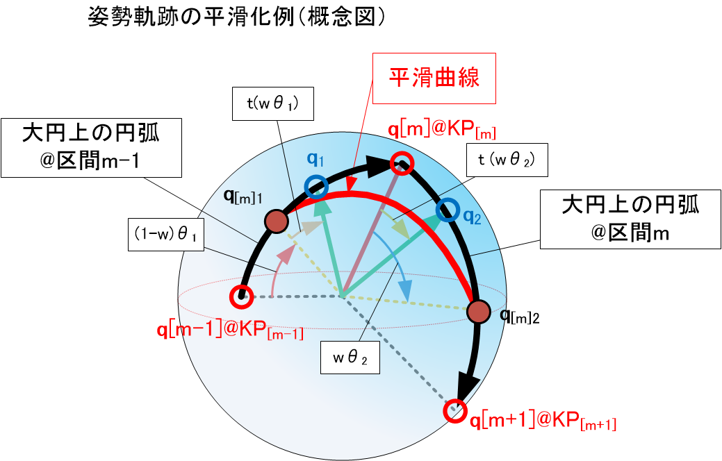
Taking KP$_{[m]}$ as the interval boundary, let $\bold q_{[m-1]}$, $\bold q_{[m]}$, $\bold q_{[m+1]}$ be the Quaternions at KP$_{[m-1]}$, KP$_{[m]}$, KP$_{[m+1]}$, respectively,

$$\begin{align*} & \bold q_{[m]1} = \rm{Slerp}(1-w, \bold q_{[m-1]}, \bold q_{[m]} ) \\ & \bold q_{[m]2} = \rm{Slerp}(w, \bold q_{[m]}, \bold q_{[m+1]} ) \end{align*}$$

is calculated. Here, $w$ is a relatively small value (about 0.3). Therefore, $\bold q_{[m]1}$ is a posture somewhat towards KP$_{m}$ in the middle of interval m-1, and $\bold q_{[m]2}$ is a posture somewhat towards KP$_{m}$ in the middle of interval m. After this, calculate the smooth posture change trajectory $\bold q$ by the following interpolation method.
That is

$$\begin{align*} & \bold q_1 = \rm{Slerp}(t, \bold q_{[m]1}, \bold q_{[m]} ) \\ & \bold q_2 = \rm{Slerp}(t, \bold q_{[m]}, \bold q_{[m]2} )　\\ & \bold q = \rm{Slerp}(t, \bold q_1, \bold q_2 )　\\ \end{align*}$$

By sequentially sampling $\bold q$ while changing the parameter t from 0 to 1, a smooth sequence of Quaternions can be obtained. Combine this with the great circle arc of interval m-1 from $\bold q_{[m-1]}$ to $\bold q_{[m]1}$ and the great circle arc of interval m from $\bold q_{[m]2}$ to $\bold q_{[m+1]}$ to form a smooth posture trajectory.

This is a method for smoothing based on a different idea from the previously mentioned smoothing. The original "vector" velocity profiles for the intervals before and after the target KP are shown in the upper part of the figure below. The left half is the usual sequence of velocity vectors when the tool tip moves along the trajectory in the backward (time-reversing direction) interval, and it is trapezoidal control. The right half is the sequence of velocity vectors in the forward (time-flowing direction) interval, and this is also trapezoidal control. If you want to make the movement smooth near the boundary where these two KPs are located, just shift the previous trapezoid and the following trapezoid and combine them. This is shown in the lower part of the figure. In this figure, the velocity vector profile is partially overlapped like velocity control. This method of interpolating the original trajectories before and after to form a smooth position/posture trajectory is called the Overlapped Velocity Method (OVV).

Here, the time to shift the forward-side trapezoid (right half) backward (leftward) is called the overlap time $t_{ov}$. The larger this is, the faster the KP area can be passed in a short time, $t_{ov}$, without reducing the speed.

Generally, as shown in the following equation, the position $\vec{P}(t)$ can be calculated by the time integral of the velocity $\vec {V}$.

$$\vec{P}(t) =\int_{ts}^{te} \vec{V}(t) dt　+\vec {P}_s$$

By utilizing this relationship well, a smooth time series representing the state of velocity overlap can be calculated from the time series of the position/posture of the original trajectory curves.

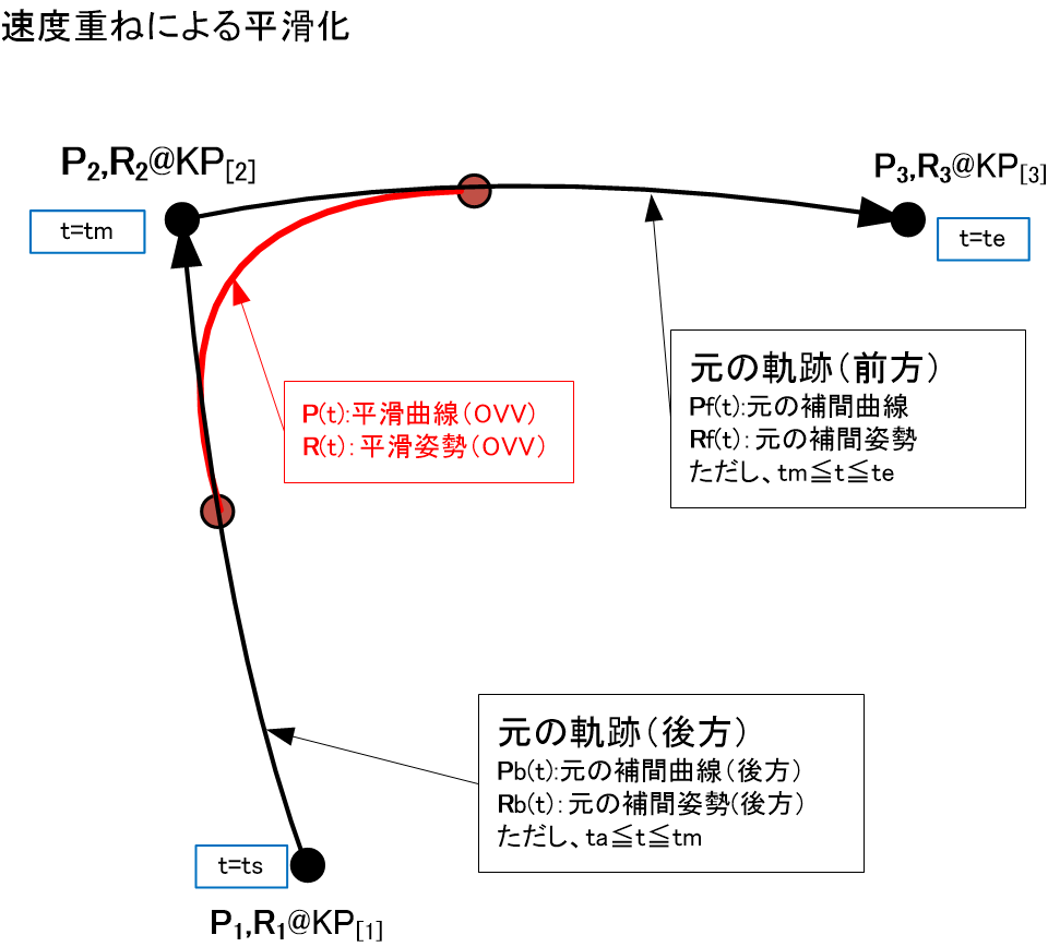
Although a specific proof is not given here, the following conclusion is obtained. In the state shown in the above figure, let $\vec{P}(t)$, $\bold{R}(t)$ be the position (3-dimensional vector) and posture (3x3 rotation matrix) at time t, respectively. Then, the interpolation formula for the trajectory in the state of velocity overlap can be simply expressed as

$$\begin{align*} &(t_m-t_{ov}) \lt t \le t_m のとき\\ &\vec{P}(t)=\vec{P}_b(t) + \vec{P}_f(t+t_{ov})- \vec {P}_2 \\ &\bold{R}(t)=\bold{R}_f(t+t_{ov})~ \bold{R}^{-1}_2~ \bold{R}_b(t) \\ \end{align*}$$

Note that $t_m$ is the time when KP$_{[2]}$(=$\vec{P}_2$, $\bold{R}_2$) is reached when following the original trajectory.

Therefore, if time series sample data is available, the following simple processing can obtain smoothing samples. If the time series of positions before and after sampled by j, $\vec{P}_f[j], \vec{P}_b[j]$, and the time series of postures before and after, $\bold{R}_f[j], \bold{R}_b[j]$, are already prepared,

$$\begin{align*} & \Delta t：Time sample width \\ & j_m：Sample point index of \vec{P}_b[j] or \bold{R}_b[j] at KP[2] \\ & ~~~~~\iff \vec{P}_b[j_m]=\vec{P}_2 and \bold{R}_b[j_m]=\bold{R}_2　\\ & nj = \rm{round}(\frac{t_{ov}}{\Delta t}) ：Number of samples for overlap time\\ \end{align*}$$

Then, the smooth part is

$$\begin{align*} & (j_m-nj) \lt j \le j_m のとき\\ & \vec{P}[j]=\vec{P}_b[j] + \vec{P}_f[j+nj]- \vec {P}_2 \\ & \bold{R}[j]=\bold{R}_f[j+nj]~ \bold{R}^{-1}_2 ~\bold{R}_b[j] \\ \end{align*}$$

This allows interpolation calculations to be performed. If you want to smooth between sections of CP control such as straight lines, arcs, and splines, these methods can be used. Also, when smoothing between sections of PTP control (joint axis primary control), the same thing can be done using $\vec{\Theta}$ instead of $\vec{P}$. Moreover, when one section is CP control and the other is PTP control, this method can be applied after unifying to one type of control trajectory.

By the way, this method also requires two trajectory data (and even time series sample data) before and after for smoothing one location at the beginning of the calculation, but eventually, part of it becomes unnecessary. Be aware of the computational load and memory burden during implementation.

I have explained practical methods for trajectory generation and smoothing near boundaries. When programming a robot arm to move, I hope I have been able to show the beginnings of the calculations performed internally to generate trajectories. In actual implementation, these algorithms are tested on actual machines, modified to add improvements, and further developed for speed and stability enhancements or to add exception handling.

Next time, I will explain about singular points, which are troublesome special postures of robot arms, and methods to avoid them.

1. Shigeki Toyama, "Robotics (Mechatronics Textbook Series)", Corona Publishing Co., Ltd. (1994)
2. R.P. Paul, translated by Tsuneo Yoshikawa, "Robot Manipulators", Corona Publishing Co., Ltd. (1984)

End