Mamezou Engineering Solutions Division, Takahiro Ishii

At Mamezou, we develop various robotics technologies. We often develop applied technologies that meet client demands using robots from other companies, but we also develop industrial robots with 6-axis or 7-axis arms, known as robot arms or manipulators, from scratch. Through this development, we generate various applied technologies and proposals. I would like to share the knowledge gained here with the readers. In this explanation, I will explain various mechanisms for controlling a 6-axis industrial vertical articulated manipulator, especially introducing fundamental algorithms and related mathematics. Understanding the technical background of ROS (Robot Operating System) will also be helpful for applying and improving robots. This time, I will explain the most basic trajectory generation process.

First, I would like to explain what the hardware to be controlled is. The figure below is a typical industrial manipulator. Modeled after a human arm, it has 5 links (bones) at the end of 6 rotary joint axes and can reproduce various hand movements. The axes are, from the bottom up,

1. Ws axis (Waist)
2. Sh axis (Shoulder)
3. Eb axis (Elbow)
4. Rt axis (Wrist Rotation)
5. Bn axis (Wrist Bending)
6. Tr axis (Wrist Turning)

They are called. (Others are called [S axis, L axis, U axis, R axis, B axis, T axis] or simply [J1 axis, J2 axis, J3 axis, ..., J6 axis].)

A tool (hand) is attached to the end of the Tr axis. For example, depending on the work purpose, it can be replaced with a welding machine, laser device, grinder, driver, drill, suction machine, gripper, camera, etc.

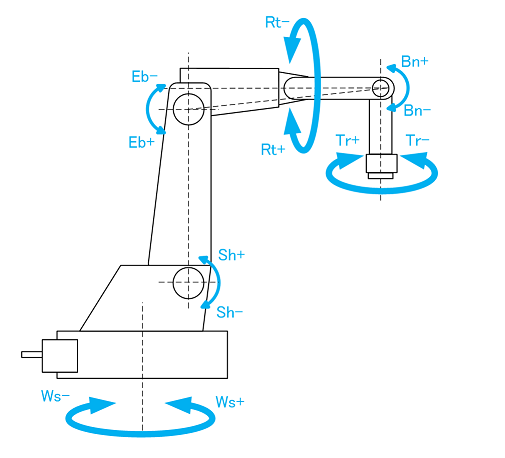
Each axis has an AC servo motor, a reducer, and a mechanical brake, which rotate to control the precise position and posture of the hand in three dimensions. By controlling the presence or absence of power, the mechanical brake can be actively released or applied. In the event of a sudden interruption of power or communication, the mechanical brake automatically applies, preventing the arm from free-falling due to its own weight.

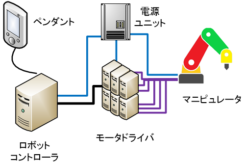
＜Motor Driver＞

It is a computer that controls the electric current to the motor so that it reaches a specified angle, specified angular velocity, or specified torque. It is designed for quick and smooth motor operation through feedback control using the rotary angle sensor in the servo motor and various signal filters. Normally, one motor driver is connected to each motor, and a total of six motor drivers are required for body control.

Each motor is connected by a communication cable for the rotary angle sensor and a power cable. The motor is powered and its own calculations are powered by a power unit.

＜Robot Controller＞

It is the main computer that comprehensively issues commands to the six motor drivers. It is also a computing device that performs various numerical calculations for the control described in this article, and is a communication I/O device such as EtherCAT, LAN, and Serial I/O. It is connected to six motor drivers via communication standards such as EtherCAT and CAN, synchronizes multiple motors, sends command values to each motor driver, and receives the actual values reached.
It also receives commands from human user interfaces (HUI) such as pendants, interprets and executes robot programs, configures environments, and records data. Furthermore, when devices for tool control are added to the robot, it also controls I/O with them and controls synchronized with robot operation.

＜Pendant＞

It is a controller that serves as an HUI. It is equipped with JOG operation buttons for instructing forward/reverse rotation for each axis and for moving and changing the posture of the hand in 3D in a straight line/circular shape. It also has functions to display, edit, and execute programs for giving complex operation instructions to the robot.

＜Power Unit＞

It distributes power to various devices from the AC power source. It transforms and becomes the AC power source for servo motors and the DC power source for peripheral devices. Since it handles large currents, it is often equipped with mechanical switches such as relays.

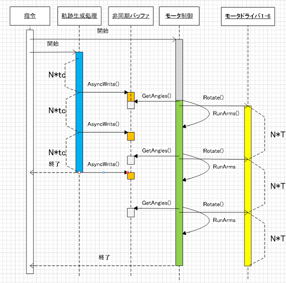
With the above configuration, the arm can be moved by repeating the following processes.

1. The robot controller calculates the joint angles $\Theta$ required for the operation for all six axes.
2. Send each angle value of the $\Theta$ element to the corresponding motor driver and execute the command.
3. The servo motors rotate and each joint moves until each commanded angle value of $\Theta$ is reached.
4. The robot controller obtains the actual angles $\Theta_{act}$ reached by each motor driver.

Here, $\Theta$ is a vector representing the joint axis angles $\theta$ between links, consisting of six elements

$$\Theta = (\theta_{1},\theta_{2},\theta_{3},\theta_{4},\theta_{5},\theta_{6} )$$

The cycle T in which the above repetition can be performed varies depending on the mechanical performance and the processing performance of the motor driver, but it is a fixed value of about 1-2 milliseconds (ms). In practice, buffering is performed, that is, multiple samples of $\Theta$ are created in advance, and sent to the motor driver all at once as asynchronous I/O. For example, if T=1[ms] and N=100 unit times, the time series $\Theta(t)(t=1\sim100)$ is sent all at once, and the actual arm operation time becomes exactly 100[ms]=0.1 second(s). If the next 100 samples of $\Theta(t)$ have been calculated and sent by this 0.1(s), continuous operation of the arm is possible without interruption. The figure below is an example of a processing sequence that realizes this.

In the next chapter, I will explain how to control the manipulator with software using this mechanism.

Generally, the geometric structure representing the positional relationship of the manipulator's links and tools is expressed in the form of DH parameters. An XYZ orthogonal coordinate system is superimposed on the joint rotation axis, and the relative state of the next joint is expressed with two distances and two angles. The table below shows the DH parameters for a PUMA-type manipulator.

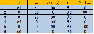
When illustrated, the figure below is obtained. All coordinate systems mentioned in this explanation are right-handed systems.

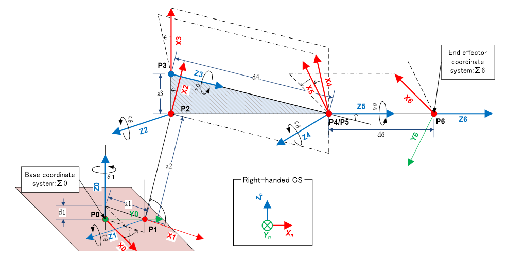
DH parameters start from the XYZ coordinate system $\Sigma_0$ of the base and proceed to the end by repeating

1. Move $d_{i}$ in the Z-axis direction
2. Rotate $θ_{i}$ around the Z-axis
3. Move $a_{i}$ in the X-axis direction
4. Rotate $α_{i}$ around the X-axis

This defines $\Sigma_i$ attached to each rotary axis. $P_i$ is the origin of $\Sigma_{i}$. $\Sigma_{6}$ is the coordinate system of the tool. Furthermore, if i=7 is added, the coordinate system $\Sigma_{7}$ of the tool tip (hand tip) $P_{7}$ can be represented. Among these, $d_i$, $a_i$, $\alpha_i$ are robot design values and constants. On the other hand, $θ_i$ is the joint axis angle, so it is a variable controlled by the servo motor.

What is the position and posture of the tool tip seen from the base coordinates when $\Theta$ is given? Let's consider how to calculate $P_7$ and $\Sigma_7$.

First, the affine transformation from $\Sigma_{i-1}$ to $\Sigma_{i}$ is expressed as a 4x4 matrix using DH parameters as follows.

$$A_i(\Theta)=\left( \begin{array}{cccc} \cos (\theta_i) & -\cos(\alpha_i)\sin(\theta_i) & \sin(\alpha_i) \sin (\theta_i) & a_i \cos (\theta_i) \\ \sin (\theta_i) & \cos(\alpha_i)\cos(\theta_i) & -\sin(\alpha_i)\cos (\theta_i) & a_i \sin (\theta_i) \\ 0 & \sin(\alpha_i) & \cos(\alpha_i) & d_i \\ 0 & 0 & 0 & 1 \\ \end{array} \right)$$

For example, in the case of $\Sigma_{1}$

$$A_1(\Theta)=A_1=\left( \begin{array}{cccc} \cos (\theta_1) & 0 & \sin (\theta_1) & a_1 \cos (\theta_1) \\ \sin (\theta_1) & 0 & -\cos (\theta_1) & a_1 \sin (\theta_1) \\ 0 & 1 & 0 & d_1 \\ 0 & 0 & 0 & 1 \\ \end{array} \right)$$

The direction of the XYZ coordinate axes and the position of the origin of $\Sigma_{i}$ seen from $\Sigma_{0}$ are calculated as

$$T_i(\Theta)=A_1 A_2 A_3 A_4 ... A_i$$

Therefore, when the coordinate system of the tool tip is $\Sigma_7$,

$$T_7(\Theta)=A_1 A_2 A_3 A_4 A_5 A_6 A_7$$

should be calculated. Here,

$$T_i(\Theta)=\left( \begin{array}{cccc} u_x & v_x & w_x & q_x \\ u_y & v_y & w_y & q_y \\ u_z & v_z & w_z & q_z \\ 0 & 0 & 0 & 1 \\ \end{array} \right)$$

If so, the upper left 3x3 submatrix $R_i$ (orthonormal system) represents the posture/direction of the coordinate system seen from the base coordinate system $\Sigma_0$, and the fourth column represents the position of the origin. That is, the direction of the 3 axes of the i-th XYZ coordinate system is

$$\vec{X_i} = ( u_x,u_y,u_z )$$

$$\vec{Y_i} = ( v_x,v_y,v_z )$$

$$\vec{Z_i} = ( w_x,w_y,w_z )$$

and the position is

$$\vec{P_i} = ( q_x,q_y,q_z )$$

It can be represented.

Here, the direction of the three axes at the tool tip is referred to as "posture", but it is cumbersome to represent it with 9 numbers, so it is represented with 3 ZYX Euler angles $(\alpha,\beta,\gamma)$. If it is rotated around the Z-axis by $\gamma$, around the Y-axis by $\beta$, and around the X-axis by $\alpha$, then

$$R_i=R_z(\gamma) R_y(\beta) R_x(\alpha)$$

Here, $R_x$ represents the 3x3 rotation matrix around the X-axis, $R_y$ around the Y-axis, and $R_z$ around the Z-axis. Solving this gives

$$\alpha=atan2(v_z, w_z);$$

$$\beta=atan2(-u_z,\sqrt{v_z^2 + w_z^2});$$

$$\gamma=atan2(u_y,u_x)$$

It can be calculated. (※atan2(y,x) is a C language function that calculates ArcTan(y/x).)

Above, the calculation to derive the position and posture of the tool tip from $\Theta$ is called forward kinematics.

One of the most important functions of a robot manipulator is to move the tool tip to a specified location with a specified posture. Therefore, contrary to the calculation of forward kinematics, it is necessary to reverse-calculate the axis angles $\Theta$ that make the position $\vec{P}$ and posture $R$ of the tool tip stand and use them as command values for the motor driver. This calculation is called inverse kinematics calculation (IK).

Represent the coordinate system of the tool tip specified by $\vec{P}$ and $R$ with the 4x4 homogeneous matrix $M_7$ and set

$$M_7=T_7(\Theta)$$

For simplicity, multiply the constant matrix $A_7^{-1}$ from the right on both sides and set

$$M_6=T_6(\Theta)$$

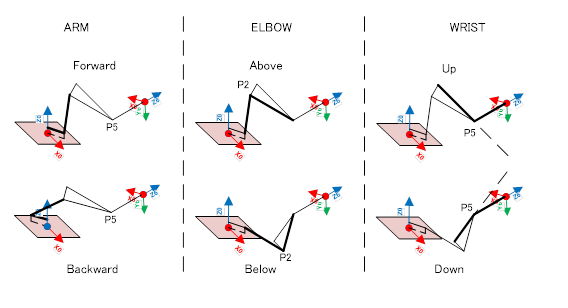
In principle, it is sufficient to solve these 12 valid elements for 6 $\theta$s. However, these are non-independent and non-linear simultaneous equations, so it is necessary to use a time-consuming algorithm such as the steepest descent method. In particular, in the case of a convergence calculation method, the number of repetitions until convergence cannot be predicted, so the calculation time becomes unstable. Therefore, IK can become a bottleneck and hinder system operation. Unlike this, analytical solution methods are known for special types of manipulators or axes. In any case, these simultaneous equations cannot be solved uniquely, and it is known that there are up to 8 combinations of solutions.

Fortunately, there is an analytical method for the 6-axis PUMA-type manipulator in this example. This is a method based on well-known methods using geometry. However, in terms of geometry, it becomes three types of two choices (ARM Forward/Backward, ELBOW Above/Below, WRIST Up/Down (see figure below)), and as a combination, there are up to $2^3=8$ possibilities of solutions.

Therefore, it is necessary to have some rational selection method, such as specifying the form, choosing the combination closest to the current value of $\Theta$, etc. Below is the core part of the IK code we actually implemented (※1) for reference.

※1. Note that this is not practical as is because details of exception handling and inspection processing are omitted.

///////////////////////////////////////////////////////////
/// @brief Find joint axis angle with inverse kinematics (IK) (holding mode setting)
///////////////////////////////////////////////////////////
int Kinematics::CalcJointAngles6ByIKwithMode(
                        const Matrix4x4& T6,
                        const JAngles6& prev_theta,
                        JAngles6& theta,
                        int mode[3],
                        double& diff_average,
                        bool bCheckRange) const
{
    JAngles6& th=theta; // angle
    JAngles6 dth; // difference between angle and prev_angle
    int ndif=0;
    diff_average=1.0e+10;
    const double &ux = T6.At(0,0), &vx = T6.At(0,1), &wx = T6.At(0,2), &qx = T6.At(0,3);
    const double &uy = T6.At(1,0), &vy = T6.At(1,1), &wy = T6.At(1,2), &qy = T6.At(1,3);
    const double &uz = T6.At(2,0), &vz = T6.At(2,1), &wz = T6.At(2,2), &qz = T6.At(2,3);

    const double &d1 = m_d1, &d4=m_d4, &d6=m_d6;
    const double &a1 = m_a1, &a2=m_a2, &a3=m_a3;
    const int mode_arm   = mode[0]; //Forward+/Backward-
    const int mode_elbow = mode[1]; //Above+/Below-
    const int mode_wrist = mode[2]; //Up+/Down- 

    //---------------------------------------------------
    // th[1]
    //---------------------------------------------------
    //P Position = O4 / O5 @ WC
    double px = qx-d6*wx;
    double py = qy-d6*wy;
    double pz = qz-d6*wz;
    int iret=0;
    double karm;

    //check Arm mode
    if(mode_arm>0){    //Arm Forward
        karm = 1.0;
    }else{            //Arm Backward
        karm = -1.0;
    }
    th[1] = atan2(karm*py, karm*px);
    iret=EvaluateAxisTheta(1, prev_theta, th, dth,  bCheckRange);
    if(iret<0) return iret;
    ndif++;

    //---------------------------------------------------
    // th[3]
    //---------------------------------------------------
    double C1=cos(th[1]);
    double S1=sin(th[1]);

    // k1*S3 + k2*C3 =k3 Solve
    double k1 = 2.0*a2*d4;
    double k2 = 2.0*a2*a3;
    double k3 = px*px +py*py +pz*pz    +a1*a1 -a2*a2 -a3*a3
                    +d1*d1 -d4*d4 -2.0*( a1*(px*C1+py*S1) + d1*pz );
    double denom1 =k2+k3;
    double t=0.0;

    // Normal solution
    // (k2+k3)*t^2 -2*k1*t +(k3-k2) =0 Solve
    double D  = k1*k1 + k2*k2 - k3*k3;
    double rootD = sqrt(D);

    ///   Elbow Mode: Above(+1)/Below(-1)
    if(mode_elbow>0){    //Above(+1)
        t = (k1-rootD)/denom1;
    }else{                //Below(-,1){    //Below(-1)
        t = (k1+rootD)/denom1;
    }
    th[3] = 2.0*atan(t);
    iret = EvaluateAxisTheta(3, prev_theta, th, dth,  bCheckRange);
    if(iret<0) return iret;
    ndif++;

    //---------------------------------------------------
    // th[2]
    //---------------------------------------------------
    double C3=cos(th[3]);
    double S3=sin(th[3]);
    //----------------------
    // myu1*C2 + nyu1*S2=gamma1
    // myu2*C2 + nyu2*S2=gamma2 Solve
    double myu1 = 	a3*C3 +d4*S3 +a2;
    double nyu1 =	d4*C3 -a3*S3;
    double gamma1 =	px*C1 +py*S1 -a1;
    double myu2 = -nyu1;
    double nyu2 =  myu1;
    double gamma2 = -d1+pz;
    double denom2 = -myu1*myu1-nyu1*nyu1;
    double C2 =  (gamma2*nyu1-gamma1*nyu2)/denom2;
    double S2 = -(gamma2*myu1-gamma1*myu2)/denom2;

    th[2] = atan2(S2,C2);
    iret=EvaluateAxisTheta(2, prev_theta, th, dth,  bCheckRange);
    if(iret<0) return iret;
    ndif++;

    //---------------------------------------------------
    // th[5]
    //---------------------------------------------------
    const double th23 = th[2]+th[3];
    const double C23 = cos(th23);
    const double S23 = sin(th23);
    double C5 = -wz*C23+(wx*C1+wy*S1)*S23;
    const double th5 = acos(C5);
    double S5  = sqrt(1.0-C5*C5);

    /// Wrist Mode: Up(+1)/Down(-1)
    if(mode_wrist>0){
        th[5] = th5;  //Wrist Up
    }else{
        th[5] = -th5; //Wrist Down
        S5  = -S5;
    }
    iret=EvaluateAxisTheta(5, prev_theta, th, dth,  bCheckRange);
    if(iret<0) return iret;
    ndif++;

    //---------------------------------------------------
    // th[4],th[6]
    //---------------------------------------------------
    const double C4 = (wx*C1*C23+wy*C23*S1+wz*S23)/S5;
    const double S4 = (-wy*C1+wx*S1)/S5;
    th[4] = atan2(S4,C4);
    iret=EvaluateAxisTheta(4, prev_theta, th, dth,  bCheckRange);
    if(iret<0) return iret;
    ndif++;

    const double C6 =  ( uz*C23-(ux*C1+uy*S1)*S23)/S5;
    const double S6 =  (-vz*C23+(vx*C1+vy*S1)*S23)/S5;
    th[6] = atan2(S6,C6);
    iret=EvaluateAxisTheta(6, prev_theta, th, dth,  bCheckRange);
    if(iret<0) return iret;
    ndif++;

    //--------------------------------
    // Average angle calculation
    double d_sum=0.0;
    double d;
    for(int i=1;i<=6;i++){
        d = dth[i]/(m_theta_upper[i] - m_theta_lower[i]);// Normalize in the operating range.
        d_sum += d*d;
    }
    diff_average = d_sum;

    return 0;
}

Let $\vec{P_t}$ be the position of the tool tip, then the following 6x6 matrix, which is the velocity transformation Jacobian matrix, can be calculated. Here " $\times$" denotes the vector product, and the superscript T denotes the transpose of the matrix.

$$J=\left( \begin{array}{ccccc} [\vec{Z_0} \times (\vec{P_t}-\vec{P_0})]^T & [\vec{Z_1} \times (\vec{P_t}-\vec{P_1})]^T & [\vec{Z_2} \times (\vec{P_t}-\vec{P_2})]^T & ... &[\vec{Z_5} \times (\vec{P_t}-\vec{P_5})]^T\\ \vec{Z_0}^T & \vec{Z_1}^T & \vec{Z_2}^T & ... & \vec{Z_5}^T\\ \end{array} \right)$$

Using this Jacobian matrix, the translational and rotational velocities of the tool tip can be calculated from the joint axis velocities as follows.

$$\Omega=( \omega_1, \omega_2 , \omega_3 , \omega_4 , \omega_5 , \omega_6 )$$

$$\left( \begin{array}{c} {\vec{v_t}^T} \\ {\vec{w_t}^T} \\ \end{array} \right) =J \Omega^T$$

Here $\omega_i$ {i=1,2,...,6} are the angular velocities of each axis, $\vec{v_t}$ is the 3D translational velocity vector of the tool tip, and $\vec{w_t}$ is the 3D rotational velocity vector.
Generally, since the inverse matrix $J^{-1}$ of $J$ can be uniquely determined,

$$\Omega^T = J^{-1} \left( \begin{array}{c} {\vec{v_t}^T} \\ {\vec{w_t}^T} \\ \end{array} \right)$$

Thus, it is also possible to determine the angular velocities of the six axes from the translational and rotational velocities of the tool tip.

These transformation formulas are often used to display the state of the robot, analyze its operation, perform mechanical calculations, and other special controls.

PTP Control and CP Control

Using the basic mathematics and algorithms described above,

• PTP (Point to Point) control = Control to move the joints by calculating the time series $\Theta(t_j)$ that can smoothly move from the current state $\Theta_{s}$ to the specified $\Theta_{e}$.
• CP (Continuous Path) control = Control to move the joints by first calculating the time series $T_7(t_j)$ so that the tool tip smoothly reaches the specified points or specified postures along a certain 3D shape (straight line, arc, etc.), and then calculating $\Theta(t_j)$ using IK.

is performed. (Here, $t_j$ indicates an equidistant time series with a sample period T=1[ms] given to the motor driver.)

The generation of such time series samples is called trajectory generation. In the case of PTP, generating a time series of $\Theta(t_j)$ is referred to, and in the case of CP, generating a time series of $T_7(t_j)$ is referred to. It is important to note that this time series must be an equal-time interval series with period T. In either case, the starting point, the endpoint, and the operating speed in between are required.

In the actual UI for specifying the trajectory, for example, in a robot program, the following specification method is used. The starting point is the current state of the robot posture, and only the endpoint is specified for each command.

20: JOINT 90,0,0,0,0,0 maxvr=30.0 
21: LINE_MOVE -400, 200, 200　maxvc=150
22: CIRCLE_MOVE  500, 300, 200　maxvc=150

These points are called KP (Key Points). In a PTP command like the JOINT command, assuming that each axis rotates straight between the starting and ending KPs, the angular velocity profile for each axis is determined so that the maximum angular velocity maxvr is reached, and the samples of $\Theta(t)$ are calculated. On the other hand, in CP commands such as LINE_MOVE and CIRCLE_MOVE, the shape of the tool tip trajectory (straight line, arc, respectively) connecting the KPs and the speed profile so that the tool tip speed reaches the maximum speed maxvc are determined, and the sample points $T_7(t)$ are first calculated. Finally, the samples of $\Theta(t)$ are calculated by IK.

Note that while the maximum speed is often specified for setting the speed profile, the travel time from the start KP to the end KP is also sometimes specified.

Method of Determining the Speed Profile

The figure below shows an example of a speed profile during CP control, showing a trapezoidal speed profile. The travel distance S between KPs is calculated from the trajectory shape. Also, $T_a$, $T_d$ are predetermined as system settings, and the maximum speed $v_c$ is specified by the user. Since the time integral of the speed (i.e., the area) becomes the travel distance, the shape of the trapezoid can be determined by adjusting it so that S becomes equal to the trapezoidal area.

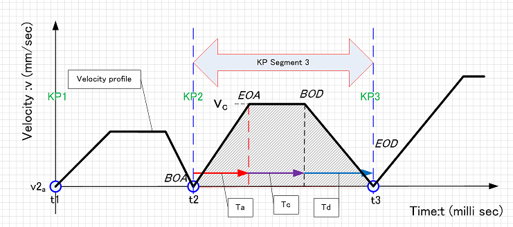
This profile is exactly trapezoidal, and at points such as BOA, EOD, EOA, and BOD, the acceleration (the first derivative of the profile) changes suddenly. Therefore, when actually moving the joints with this, mechanical shocks and vibrations often occur in the vicinity. To operate smoothly without vibrations, this area is often connected with a smooth curve using higher-order functions or trigonometric functions to smooth it out. At this time, care is taken to ensure that the area is the same as the trapezoidal area S.

Trajectory Sampling

The shape of the trajectory specified for CP control can be analytically determined using geometry. That is, it can be concretely calculated as a series of $T_7(s_k)$ {k=0,1,2...} with an appropriate parameter $s_k$. However, the series $T_7(s_k)$ is clearly different from the required equal-time sampling series $T_7(t_j)$. How should this difference be corrected to sample the correct time series?

This difference arises from the difference between the parameters $s_k$ and $t_j$. The figure below shows the graph obtained by integrating the speed profile, with the vertical axis being the travel distance $S(t)$. It is a monotonically increasing curve as time progresses.

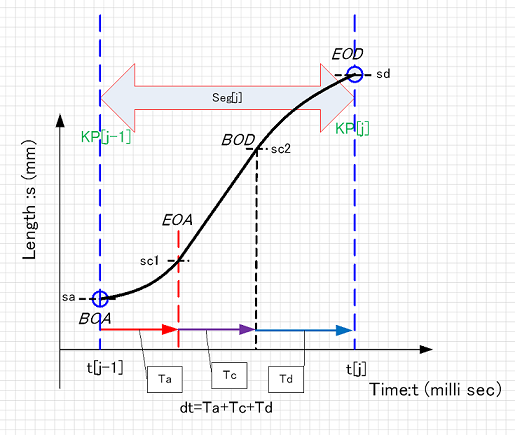
On the other hand, the travel distance samples $S'(s_k)$ can be geometrically calculated from $T_7(s_k)$, which is also a monotonically increasing function with respect to $s_k$. In this case, it is a function independent of time. If the trajectory shape is complex, it may be a curve, but it is still a monotonically increasing function. Ultimately, both $S$ and $S'$ are one-to-one relationships with respect to the parameter. Therefore, it is possible to correspond the parameters $s$ and $t$ via the travel distance $S$. That is, the following processing is possible.

1. Calculate the value of $S(t_{j})$.
2. Reverse the table $s_{k}$ ⇒ $S'(s_{k})$ and view it as a table $S'(s_{k})$⇒ $s_k$. From this table, interpolate the value $S(t_j)$ to obtain the value $s_{intp}$ (linear interpolation is sufficient).
3. Calculate $T_7(s_{intp})$. Set this as $T_7(t_{j})$.

Repeat the above for $j=0,1,2,..$ until the end KP is reached, and if the time series $T_7(t_j)$ can be generated, the trajectory generation is completed. In the case of PTP control, the same processing can be performed using a representative $\theta_i$ (※2) instead of S. Also, in the case of CP control, the obtained $T_7(t_j)$ can be converted by IK to obtain the joint angle series $\Theta(t_j)$ necessary for motor control.

※2. For example, the one that performs the largest operation among the six $\theta$s.

Starting from the structure of the manipulator, after introducing the basic ideas and mathematics required for its control, I explained the method of trajectory generation for actually operating it. However, the following regarding CP control was not described in detail in the above explanation.

• What is the specific method for geometrically sampling the trajectory? For example, how are commonly used straight trajectory, circular trajectory, and spline trajectory calculated using $s_k$?
• How is the change in posture (rotation) of the tool tip sampled?
• There are special postures of the arm, or combinations of $\theta_i$, called "singular points", which become problems in control. What are they, and how should they be avoided?

I would like to explain these in the next session.

1. Shigeki Toyama, "Robotics (Mechatronics Textbook Series)", Corona Publishing (1994)
2. R.P. Paul, "Robot Manipulators", translated by Tsuneo Yoshikawa, Corona Publishing (1984)

End