使用最优化库CeresSolver解决非线性最小二乘问题
Back to Top为了覆盖更广泛的受众,这篇文章已从日语翻译而来。
您可以在这里找到原始版本。
本文是is开发者网站Advent日历2025第10天的文章。
0. 引言
#在机器人控制和图像处理领域,常常需要求解优化问题。
所谓优化问题,也有线性规划、组合优化等多种类型和求解方法。
其中,在实际应用中尤其常见的是“最小二乘问题”。
这是求解如下目标函数 的最小值参数 的问题。
(通常, 为向量。)
这里,上式中的 称为残差(Residual),表示观测数据(=实测值) 与预测值(=理论值) 之差。
这次将介绍 Google 出品的求解器 “Ceres Solver” ,它能高效地解决这种非线性最小二乘问题。
1. 本文的环境
#本文以 Ubuntu 24.04 为目标。
作者环境使用 WSL2,但原生 Ubuntu 上也不存在问题。
本文在 Ubuntu 环境中使用该库,但在 Windows 上也可运行。
详情请参阅下方链接:
http://ceres-solver.org/installation.html#windows
2. 环境搭建
#这是使用 CeresSolver 的前期准备。内容稍长,敬请耐心阅读。
安装所需库
#首先,安装构建 Ceres Solver 所需的工具。
按下面每行命令依次执行,完成安装。
# apt update(会提示输入密码)
sudo apt update && sudo apt upgrade -y
# 构建工具
sudo apt install build-essential
# Git
sudo apt install git
# CMake
sudo apt install cmake
# google-glog + gflags
sudo apt install libgoogle-glog-dev libgflags-dev
# 使用 ATLAS 提供 BLAS & LAPACK
sudo apt install libatlas-base-dev
# Eigen3
sudo apt install libeigen3-dev
# SuiteSparse(可选)
sudo apt install libsuitesparse-dev
创建工作空间
#接下来,在任意位置创建一个工作空间。
这里以在主目录下创建 ceres_solver_ws 目录为例。
mkdir ~/ceres_solver_ws
在一般的 Linux 环境中,"~"(波浪号)表示主目录。
主目录的绝对路径为 /home/${用户名}/。
克隆 CeresSolver 库
#工作空间创建好后,克隆 CeresSolver 源码。
克隆位置任意,此处在 external 目录下进行。
由于需要递归地获取 Submodule,请务必添加 --recursive 选项。
cd ~/ceres_solver_ws
mkdir external
cd external
git clone --recursive https://github.com/ceres-solver/ceres-solver
也可以使用 --recurse-submodules 选项来递归获取子模块:
git clone --recurse-submodules ${repo-url}
构建并安装 CeresSolver 库
#克隆完成后,使用 CMake 进行构建。
# 进入 CeresSolver 源码目录
cd ceres-solver
# 创建用于构建的目录
mkdir build
# 生成构建系统(源外构建)
cmake -S . -B build
# 执行构建
cmake --build build
如果执行命令时出现以下错误,请通过 apt 安装 build-essential 包。
CMake Error at CMakeLists.txt:33 (project):
  No CMAKE_CXX_COMPILER could be found.

  Tell CMake where to find the compiler by setting either the environment
  variable "CXX" or the CMake cache entry CMAKE_CXX_COMPILER to the full path
  to the compiler, or to the compiler name if it is in the PATH.

-- Configuring incomplete, errors occurred!
构建需要一些时间。可通过下面命令使用并行作业来加速。
nproc 命令用于“获取系统可用 CPU 核心数”。
该命令的输出会替换 $(nproc)。
cmake --build build -- -j$(nproc)
如果日志显示如下且进度达到 100%,则表示构建成功:
[ 99%] Built target robot_pose_mle
[ 99%] Building CXX object examples/sampled_function/CMakeFiles/sampled_function.dir/sampled_function.cc.o
[ 99%] Linking CXX executable ../../bin/sampled_function
[ 99%] Built target sampled_function
[ 99%] Building CXX object examples/slam/pose_graph_2d/CMakeFiles/pose_graph_2d.dir/pose_graph_2d.cc.o
[ 99%] Linking CXX executable ../../../bin/pose_graph_2d
[ 99%] Built target pose_graph_2d
[ 99%] Building CXX object examples/slam/pose_graph_3d/CMakeFiles/pose_graph_3d.dir/pose_graph_3d.cc.o
[100%] Linking CXX executable ../../../bin/pose_graph_3d
[100%] Built target pose_graph_3d
最后,将构建产物安装到系统中。
默认安装路径为 /usr/local。
# 安装构建产物
sudo cmake --install build
安装完成后,为保险起见,执行以下命令:
source ~/.bashrc
3. 尝试简单的优化计算
#创建 CMakeLists.txt 和源文件
#现在,使用 CeresSolver 实际求解一个优化问题。
首先,返回工作空间 ~/ceres_solver_ws,创建 CMakeLists.txt 文件。
cd ~/ceres_solver_ws
touch CMakeLists.txt
在 CMakeLists.txt 中写入以下内容。编辑器自选,此处使用 Visual Studio Code。
(与 WSL 兼容性良好,推荐使用!)
# 指定 CMake 最低版本
cmake_minimum_required(VERSION 3.14)

# 定义项目名
project(ceres-solver-sample)

# 设置可执行文件输出到构建目录根下
# (不需要可删除此行)
set(CMAKE_RUNTIME_OUTPUT_DIRECTORY ${CMAKE_BINARY_DIR})

# 依赖包
find_package(Ceres REQUIRED)

# 添加子目录
add_subdirectory(src)
接着,在工作空间根目录创建 src 目录,并在其中创建 CMakeLists.txt:
cd ~/ceres_solver_ws
mkdir src
cd src
touch CMakeLists.txt
在 src/CMakeLists.txt 中写入:
# simple-ols
add_executable(simple-ols simple-ols.cpp)
target_link_libraries(simple-ols absl::log_initialize Ceres::ceres)
最后,创建主程序文件 simple-ols.cpp,文件名须与上面一致:
touch simple-ols.cpp
最终文件结构如下:
ceres_solver_ws/
├── CMakeLists.txt
└── src/
    ├── CMakeLists.txt
    └── simple-ols.cpp
实现优化计算
#在 simple-ols.cpp 中编写以下内容。
此次示例中,我们求解如下函数 的最小值点 :
显然 时取得最小值,但我们通过程序来计算。实现代码如下:
#include <ceres/ceres.h>
#include <glog/logging.h>

using ceres::AutoDiffCostFunction;
using ceres::CostFunction;
using ceres::Problem;
using ceres::Solver;

/// @brief 残差结构体
/// @remark 在()运算符中描述优化目标
struct CostFunctor
{
    template <typename T>
    bool operator()(const T* const x, T* residual) const
    {
        // 本次优化目标式
        residual[0] = T(5.0) - x[0];
        return true;
    }
};

/// @brief 主函数
int main(int argc, char** argv)
{
    // 定义初始值
    double initial_x = 1.0;
    double x = initial_x;

    // 定义代价函数
    CostFunction* cost_function = new ceres::AutoDiffCostFunction<CostFunctor, 1, 1>();

    // 定义优化问题
    Problem problem;
    problem.AddResidualBlock(cost_function, nullptr, &x);   // 添加残差块
    problem.SetParameterLowerBound(&x, 0, 0.0);             // 设置输入参数下限
    problem.SetParameterUpperBound(&x, 0, 10.0);            // 设置输入参数上限

    // 定义计算选项
    ceres::Solver::Options options;
    options.linear_solver_type = ceres::DENSE_QR;           // 使用稠密矩阵的QR分解
    options.minimizer_progress_to_stdout = true;            // 启用进度输出
    options.max_num_iterations = 10;                        // 最大迭代次数

    // 定义计算结果
    Solver::Summary summary;

    // 执行优化计算
    ceres::Solve(options, &problem, &summary);

    // 输出计算结果
    // 计算结果存储在变量 x 中
    std::cout << summary.BriefReport() << std::endl;
    std::cout << "x: " << initial_x << " -> " << x << std::endl;

    return 0;
}
程序详情
#以下说明代码中重要部分。
代价定义
#/// @brief 代价结构体
/// @remark 在()运算符中描述优化目标
struct CostFunctor
{
template <typename T>
bool operator()(const T* const x, T* residual) const
{
// 本次优化目标式
residual[0] = T(5.0) - x[0];
return true;
}
};
在 () 运算符中描述此次优化的目标式。
- 必须在
()运算符内部编写计算式。 - 模板参数
T会被用于优化计算时的类型。- 具体来说,使用的是名为
ceres::Jet的数据类型。 - 如果使用
double等类型,需要注意将其转换为T类型。
- 具体来说,使用的是名为
代价函数定义
#// 定义代价函数
CostFunction* cost_function = new ceres::AutoDiffCostFunction<CostFunctor, 1, 1>();
上述代码定义了代价函数,本例中使用自动微分(Automatic Differentiation)。
模板参数含义如下:
- 第1个模板参数:代价函数的结构体类型
- 第2个模板参数:误差(残差)参数的维度
- 第3个模板参数:优化参数的维度
本例中,因误差参数()为标量,其维度为 1;优化参数 亦为标量,维度同为 1。
优化问题定义
#// 定义优化问题
Problem problem;
problem.AddResidualBlock(cost_function, nullptr, &x); // 添加残差块
problem.SetParameterLowerBound(&x, 0, 0.0); // 设置输入参数下限
problem.SetParameterUpperBound(&x, 0, 10.0); // 设置输入参数上限
在此定义优化问题,并设置输入参数的上下限。
AddResidualBlock 方法的第2个参数可用于定义损失函数(Loss Function)。
本文不做深入介绍,详情请参阅:
http://ceres-solver.org/nnls_tutorial.html#robust-curve-fitting
构建与运行
#使用 CMake 构建刚才编写的程序:
cd ~/ceres_solver_ws
cmake -S . -B bin
cmake --build bin
构建成功后,执行:
./bin/simple-ols
会输出类似以下日志:
iter      cost      cost_change  |gradient|   |step|    tr_ratio  tr_radius  ls_iter  iter_time  total_time
   0  8.000000e+00    0.00e+00    4.00e+00   0.00e+00   0.00e+00  1.00e+04        0    1.35e-05    4.40e-05
   1  7.998400e-08    8.00e+00    4.00e-04   0.00e+00   1.00e+00  3.00e+04        1    8.09e-05    1.88e-04
   2  8.886518e-17    8.00e-08    1.33e-08   4.00e-04   1.00e+00  9.00e+04        1    3.24e-05    2.39e-04
Ceres Solver Report: Iterations: 3, Initial cost: 8.000000e+00, Final cost: 8.886518e-17, Termination: CONVERGENCE
x: 1 -> 5
从最后一行日志可得最优输入值为 5。
此外,在最优输入下的残差代价(Final cost)为 8.886518e-17,几乎为 0。
尝试更改输入参数的上下限
#接下来,将输入值范围改为 1~3 再运行试试。
将以下 ★ 标注处的值从 10 改为 3。
// 定义优化问题
Problem problem;
problem.AddResidualBlock(cost_function, nullptr, &x);   // 添加残差块
problem.SetParameterLowerBound(&x, 0, 0.0);   // 设置输入参数下限
problem.SetParameterUpperBound(&x, 0, 3.0);   // 设置输入参数上限(★)
重新构建并运行后,可见最优输入为 ,残差代价为 2.000000e+00。
这表明在指定的约束范围内,优化器找到了使代价最小的输入值。
参考日志如下:
iter      cost      cost_change  |gradient|   |step|    tr_ratio  tr_radius  ls_iter  iter_time  total_time
   0  8.000000e+00    0.00e+00    2.00e+00   0.00e+00   0.00e+00  1.00e+04        0    1.21e-05    4.23e-05
   1  2.000000e+00    6.00e+00    0.00e+00   0.00e+00   7.50e-01  1.14e+04        1    6.80e-05    1.66e-04
Ceres Solver Report: Iterations: 2, Initial cost: 8.000000e+00, Final cost: 2.000000e+00, Termination: CONVERGENCE
x: 1 -> 3
4. 使用数值方法求解4自由度平面机械臂的逆运动学
#第3章展示了解决输入参数与代价均为标量的优化问题的示例。本章作为更复杂的非线性优化案例,将求解“4自由度平面机械臂的逆运动学”。
什么是4自由度平面机械臂
#下面以如图所示具有 4 个关节的平面机械臂为对象,实现逆运动学计算。
参数定义如下:
- 各连杆长度记为
- 各关节的转角记为
- 各关节的正转方向为“逆时针(ccw)”
- 机器人末端(点 P)的 X 坐标为 ,Y 坐标为
- 机器人末端的姿态角(射线 CP 与 X 轴的夹角)记为
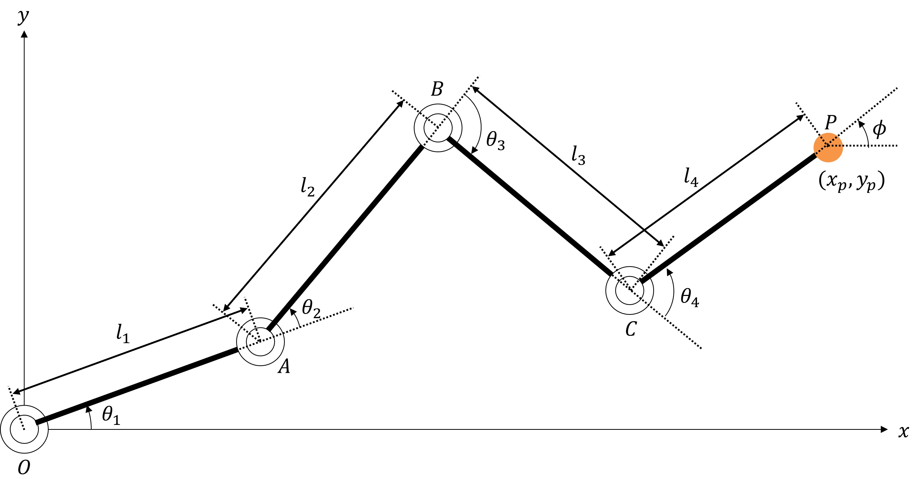
正运动学计算
#考虑目标机器人各关节角 与末端位置 的关系。
此处,各向量定义如下:
如上图,从原点 O 到点 A 的向量 表示为:
同理,从点 A 到点 B、点 B 到点 C、点 C 到点 P 的向量分别为:
将以上向量相加后,点 P 在 XY 平面上的坐标为:
此外,机器人末端的姿态角 为:
结合上述两个公式,将从关节角向量 到末端位置向量 的映射定义为 ,则:
这就是进行正运动学计算时使用的公式。
逆运动学计算
#另一方面,逆运动学(Inverse Kinematics)顾名思义即正运动学的逆运算。
也就是说,求取 的逆函数(即从末端位置 到关节角 的映射):
通常逆运动学计算的计算量比正运动学更多。
根据机器人结构,有时可解析求解,但一般自由度越多,逆运动学求解难度越高。
这次我们将使用 CeresSolver 对该计算进行数值求解。
代码实现
#目录与 CMakeLists.txt 的创建
#在 src 目录下创建存放本问题文件的子目录 4dof-ik:
cd ~/ceres_solver_ws/src
mkdir 4dof-ik
cd 4dof-ik
touch CMakeLists.txt
然后在 src/CMakeLists.txt 的末尾添加:
# simple-ols
add_executable(simple-ols simple-ols.cpp)
target_link_libraries(simple-ols absl::log_initialize Ceres::ceres)

# 注册 4dof-ik 目录为子目录
add_subdirectory(4dof-ik)
数据结构体定义
#首先定义用于汇总数据的结构体。
在 4dof-ik 目录下创建 Pose.hpp 和 KinematicsParameters.hpp:
cd ~/ceres_solver_ws/src/4dof-ik
touch Pose.hpp
touch KinematicsParameters.hpp
在 Pose.hpp 中写入:
/// @brief 位姿
struct Pose
{
    /// @brief X坐标
    double x;

    /// @brief Y坐标
    double y;

    /// @brief 末端角度
    double phi;

    Pose(double x_, double y_, double phi_)
        : x(x_), y(y_), phi(phi_) {}
};
在 KinematicsParameters.hpp 中写入:
/// @brief 机械结构参数(连杆长度)
struct KinematicParameters {
    /// @brief 第1连杆长度
    double L1;

    /// @brief 第2连杆长度
    double L2;

    /// @brief 第3连杆长度
    double L3;

    /// @brief 第4连杆长度
    double L4;

    /// @brief 构造函数
    /// @param l1 第1连杆长度
    /// @param l2 第2连杆长度
    /// @param l3 第3连杆长度
    /// @param l4 第4连杆长度
    KinematicParameters(double l1, double l2, double l3, double l4)
        : L1(l1), L2(l2), L3(l3), L4(l4) {}
};
实现优化计算
#创建主程序 4dof-ik.cpp:
touch 4dof-ik.cpp
最终文件结构如下:
ceres_solver_ws/
├── CMakeLists.txt
└── src/
    ├── CMakeLists.txt
    ├── simple-ols.cpp
    └── 4dof-ik/
        ├── CMakeLists.txt
        ├── 4dof-ik.cpp
        ├── KinematicsParameters.hpp
        └── Pose.hpp
在 4dof-ik.cpp 中编写:
#include <iostream>
#include <ceres/ceres.h>
#include <ceres/rotation.h>
#include <cmath>
#include "Pose.hpp"
#include "KinematicsParameters.hpp"

/// @brief 执行正运动学
/// @tparam T 数据类型
/// @param[in] kp 机械结构参数
/// @param[in] theta 关节角度向量(数组)
/// @param[out] x X坐标
/// @param[out] y Y坐标
/// @param[out] phi 末端角度
template <typename T>
void compute_forward_kinematics(const KinematicParameters& kp, const T* const theta, T& x, T& y, T& phi)
{
    x = T(kp.L1) * cos(theta[0])
      + T(kp.L2) * cos(theta[0] + theta[1])
      + T(kp.L3) * cos(theta[0] + theta[1] + theta[2])
      + T(kp.L4) * cos(theta[0] + theta[1] + theta[2] + theta[3]);

    y = T(kp.L1) * sin(theta[0])
      + T(kp.L2) * sin(theta[0] + theta[1])
      + T(kp.L3) * sin(theta[0] + theta[1] + theta[2])
      + T(kp.L4) * sin(theta[0] + theta[1] + theta[2] + theta[3]);

    phi = theta[0] + theta[1] + theta[2] + theta[3];
}

/// @brief 代价
struct IKCostFunction
{
    Pose target_pose;
    KinematicParameters kp;

    /// @brief 构造函数
    /// @param pose 末端位置与姿态
    /// @param param 机械结构参数
    IKCostFunction(const Pose& pose, const KinematicParameters& param)
        : target_pose(pose), kp(param)
    {
    }

    template<typename T>
    bool operator()(const T* const theta, T* residuals) const
    {
        T x, y, phi;
        compute_forward_kinematics(kp, theta, x, y, phi);

        residuals[0] = T(target_pose.x) - x;   // X坐标误差
        residuals[1] = T(target_pose.y) - y;   // Y坐标误差
        residuals[2] = T(target_pose.phi) - phi;   // 姿态角误差

        return true;
    };
};

/// @brief 主函数
int main(int argc, char** argv)
{
    // 定义机械结构参数
    double l1 = 1.5;
    double l2 = 1.5;
    double l3 = 1.0;
    double l4 = 1.0;

    // 定义目标位置与姿态
    double x_target = 3.2;
    double y_target = 0.8;
    double phi_target = -M_PI_4;

    // 设置初始值
    double theta[4] = {0.0, 0.0, 0.0, 0.0};
    KinematicParameters kp(l1, l2, l3, l4);
    Pose target_pose{ x_target, y_target, phi_target };

    // 定义优化问题
    ceres::Problem problem;
    problem.AddResidualBlock(
        // 误差维度为3,优化变量维度为4
        new ceres::AutoDiffCostFunction<IKCostFunction, 3, 4>(
            new IKCostFunction(target_pose, kp)
        ),
        nullptr,
        theta
    );

    // 应用上下限值(设置为 -pi ~ pi)
    for (int i = 0; i < 4; i++)
    {
        problem.SetParameterLowerBound(theta, i, -M_PI);
        problem.SetParameterUpperBound(theta, i, M_PI);
    }

    // Solver 设置
    ceres::Solver::Options options;
    options.linear_solver_type = ceres::DENSE_QR;
    options.minimizer_progress_to_stdout = true;
    options.max_num_iterations = 100;     // 最大迭代次数
    options.function_tolerance = 1e-6;    // 收敛判定阈值

    // 执行优化计算
    ceres::Solver::Summary summary;
    ceres::Solve(options, &problem, &summary);

    // 输出计算结果
    std::cout << summary.BriefReport() << std::endl;
    if (summary.termination_type == ceres::CONVERGENCE)
    {
        std::cout << "✅ IK Solution Found! (Final Cost: " << summary.final_cost << ")\n";
    }
    else
    {
        std::cout << "❌ IK Failed to Converge.\n";
    }

    // 输出求得的关节角度
    std::cout << "theta[0] = " << theta[0] << std::endl;
    std::cout << "theta[1] = " << theta[1] << std::endl;
    std::cout << "theta[2] = " << theta[2] << std::endl;
    std::cout << "theta[3] = " << theta[3] << std::endl;

    // 验证通过求得的关节角度对应的位置与姿态
    std::cout << "Check Forward kinematics calculation:" << std::endl;
    double x_result, y_result, phi_result;
    compute_forward_kinematics(kp, theta, x_result, y_result, phi_result);
    std::cout << "x   = " << x_result << std::endl;
    std::cout << "y   = " << y_result << std::endl;
    std::cout << "phi = " << phi_result << std::endl;
    return 0;
}
添加到 CMakeLists.txt
#在 4dof-ik 目录下的 CMakeLists.txt 中添加:
# 4dof-ik
add_executable(4dof-ik 4dof-ik.cpp)
target_link_libraries(4dof-ik absl::log_initialize Ceres::ceres)
构建与运行
#进入工作空间并构建:
cd ~/ceres_solver_ws
cmake --build bin
执行:
./bin/4dof-ik
你会得到如下结果(省略迭代日志):
Ceres Solver Report: Iterations: 7, Initial cost: 2.248425e+00, Final cost: 4.808292e-20, Termination: CONVERGENCE
✅ IK Solution Found! (Final Cost: 4.80829e-20)
theta[0] = -0.414376
theta[1] = 1.25568
theta[2] = 0.609086
theta[3] = -2.23579
Check Forward kinematics calculation:
x   = 3.2
y   = 0.8
phi = -0.785398
由于最终代价几乎为 0,成功找到了满足指定目标位置与姿态的关节角度!
同时,验算结果也正确!
5. 结束语
#本文介绍了使用 CeresSolver 求解优化问题的示例程序。
除了本文示例外,官方页面还提供了许多示例程序。
有兴趣的读者可前往查看:
http://ceres-solver.org/nnls_tutorial.html#non-linear-least-squares
此外,本次编写的程序已在以下仓库开源:
https://github.com/hayat0-ota/CeresSolver_tutorial