Introduction to Reinforcement Learning for Robot Developers
Back to TopTo reach a broader audience, this article has been translated from Japanese.
You can find the original version here.
Introduction
#In this article, we will explain the fundamental theories of reinforcement learning and how to put them into practice while tackling the classic inverted pendulum problem familiar in the field of control. Although many introductory articles on reinforcement learning use examples like maze exploration programs or slot machines, for those interested in controlling robots or machinery—or considering applications in those areas—a problem like the inverted pendulum might be more intuitive.
Overview of the CartPole Task
#In this article, we will tackle the CartPole task provided by Gymnasium[1].
In this task, the goal is to keep the pole balanced by applying forces to the cart from the left or right. If the pole tilts beyond a certain angle or if the cart goes off the edge of the screen, the episode ends immediately as a failure. In reinforcement learning, the period from the start to the finish of the task is referred to as an episode. The GIF above shows an incompletely trained state where episodes end quickly and are retried repeatedly.
States and Actions
#The information observed from the system is called the state. The table below shows the elements of the state in this system along with the conditions for ending an episode.
| State Element | Episode Termination Condition | |
|---|---|---|
| 0 | Cart Position | Terminates if or |
| 1 | Cart Velocity | - |
| 2 | Pole Angle | Terminates if or |
| 3 | Pole Angular Velocity | - |
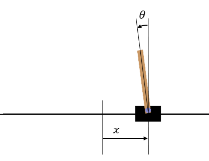 Coordinate axes for CartPole. The origin for x is at the center of the screen, and 0° for θ is in the upward direction.
In reinforcement learning, the inputs to the system are called actions. In the CartPole task, you can choose either “push the cart to the left” or “push the cart to the right.” Since the force applied is constant, it cannot be finely adjusted like in PID control. Note that with different techniques than those covered in this article, it is also possible to handle actions with variable magnitudes.
Unlike maze or slot machine tasks, control tasks require attention to the control cycle. In the CartPole task, the default control cycle is set to 0.02 seconds, and at each cycle, the state is obtained and an action is selected.
How Learning Works
#From here on, we will consider solving the CartPole task using reinforcement learning. In reinforcement learning, the entity that decides on actions is called the agent, and the object that the agent manipulates is called the environment.

The goal of reinforcement learning is to learn to select the optimal actions based on the observed state. The function that maps states to actions is called the policy, denoted by .
Rewards and Returns
#Here, we explain the important concepts of rewards and returns in reinforcement learning.
A reward is a numerical value that the agent receives from the environment at each step, serving as an indicator of how “good” its action was at that moment. The function used to calculate the reward is called the reward function, and usually the developer needs to design a reward function that fits the task. In the tasks provided by Gymnasium, the reward function is predefined, so we will use that. In the CartPole task, a reward of 1 is given at each step as long as the pole remains upright.
The return is the total sum of rewards that the agent receives, including those from future steps. If the reward obtained at step is denoted by , the return is expressed as follows:
Here, is called the discount factor, and it takes a value between 0 and 1. The discount factor serves to prevent the return from diverging.[2]
The relation between reward and return can be compared to the relationship between annual income and lifetime earnings. Although each action yields a reward (annual income), it is important not to be dazzled by immediate gains. The agent selects actions that maximize the return (lifetime earnings), which is a longer-term measure. Due to the influence of the discount factor, rewards received sooner are valued higher, while rewards obtained later are estimated to have a lower value.
Choosing Actions Using Value Functions
#In reinforcement learning, the agent learns to select actions that maximize the return. However, to calculate the return precisely, future rewards are needed. Therefore, the expected value of the return is used to select actions. The function that computes this expected return is called the value function.
State Value Function and Action Value Function
#There are two types of value functions: the state value function, which takes only the state as an argument, and the action value function, which takes both the state and the action as arguments. The state value function, , is defined in terms of the return and the current state as follows:
Similarly, the action value function, , is expressed using the chosen action as follows:
Here, denotes the expected value of the return .
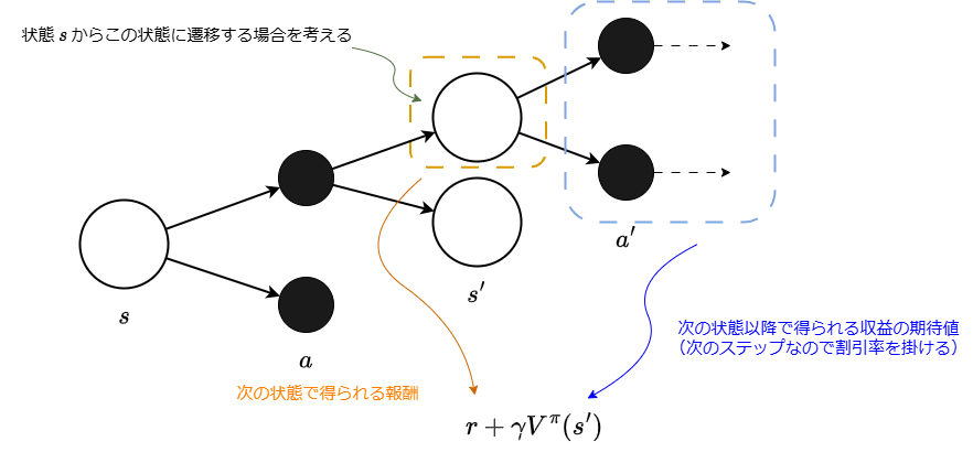
Now, to consider the specific form of the state value function, we introduce the backup diagram. The backup diagram uses white circles to represent states and black circles to represent actions, illustrating the stochastic state transitions. In reinforcement learning, both the selection of actions and the subsequent state transitions are treated as stochastic processes.[3] The diagram below shows a backup diagram in which an action is selected in state , and the system transitions to the subsequent state .
![]()
To calculate the expected value, we compute the product of the “resulting value” and its probability of occurrence, and then sum the results. Here, the “resulting value” refers to the return achieved when transitioning to a certain state . Moreover, because there are two stochastic factors—the policy and the state transition—when moving from state to state , we need to sum over both.
First, consider the “resulting value.” As shown in the diagram below, when an action is selected in a state , and the system transitions to the next state , the return can be expressed as:
This expression separates the reward obtained in state from the subsequent return.
Now that the “resulting value” is determined, we calculate the expected value by taking into account the probability of occurrence. When an action is chosen in state , the expected return from the potential next states is given by using the state transition probability as follows:
This expression represents the expected return when a particular action is chosen. By considering all possible actions through the policy —the probability of selecting action in state —we get:
This equation is called the Bellman equation and is one of the fundamental concepts in reinforcement learning. In summary, the Bellman equation comprises the following elements:
- : stochastic policy
- : state transition probability
- : reward received when transitioning from to
- : expected return from the next step onward multiplied by the discount factor
Similarly, by applying the same reasoning to the action value function , we obtain:
Simplifying for CartPole
#The Bellman equation above models both the policy and the state transitions as stochastic processes. However, in the CartPole task, the state after an action is uniquely determined (i.e., deterministic), allowing us to simplify the equation.
The simplified backup diagram and action value function are as follows:
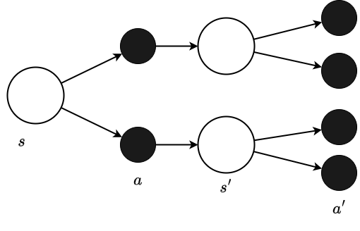
Unlike the prior backup diagram, the state following the action is unique.
Choosing Actions Using the Action Value Function
#The purpose of introducing the value function was to enable the selection of actions that yield higher returns. Since the output of the action value function represents the expected return when taking action in state , it helps determine which action to select.
Note: Choosing actions based on comparing state values is just one example of a reinforcement learning approach. Such methods are known as value-based methods.
Visualizing Part of the Value Function
#We have explained the value function, but to deepen our understanding, let’s examine a graph of this function. Rather than capturing the entire function precisely, we will focus on the expected return for a particular state.
Here, we consider the following two states:
- The state where the pole is stably upright.
- The state just before the pole falls.
First, consider the state where the pole is stably upright. In other words, this is a state where the agent can continue receiving rewards in the subsequent steps. Let’s reiterate the formula for return:
In this formula, rewards are summed over an infinite number of steps, which represents the scenario where the episode continues indefinitely. If the pole falls before that, the return is the sum of rewards up to that step. When rewards are received for steps, the return is as shown in the graph below.
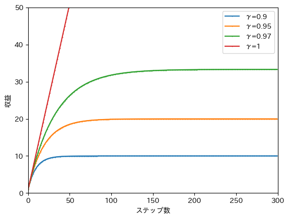
Due to the effect of the discount factor, the return converges. The converged value, however, depends on the discount factor. For example, if we adopt a discount factor of , the orange line shows that the return converges to about 20 when an episode lasts for more than 100 steps.
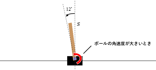
Next, consider the value just before the episode terminates when balance is lost. In the diagram below, consider a state where the pole angle is slightly inside the termination line of and has a large angular velocity directed toward crossing that line. From this state, the system transitions to the next state. (Although it does not affect the result, the calculation assumes that each action is selected with a 50% probability.)
The state value in this case is computed as follows:
Here, is the reward received when transitioning to the next state . According to the specifications of CartPole, even if the next state meets the termination conditions, a reward of 1 is still obtained. The expected return from subsequent steps, , is 0 since meets the termination condition regardless of the selected action, and no further state transitions occur. As a result, the state value of in the diagram is 1.
Now, let’s consider the form of the value function, which is our main focus. Note that the state , which is the argument of the state value function, is a 4-dimensional vector, making intuitive visualization challenging. To provide a rough idea, we will plot the return as a function of only the pole angle, while fixing the cart position, cart velocity, and pole angular velocity at 0.
With a discount factor of , the state value function looks as follows.[4]
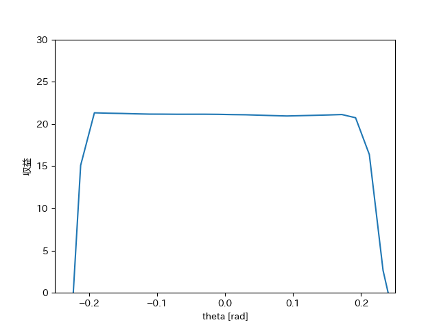
Around , where the pole is stably upright as mentioned, the return is about 20. Near the termination boundaries of (), the value decreases.
Approximating the Action Value Function with a Neural Network
#When applying the action value function to the CartPole task, further ingenuity is required. In the equations above, the state was represented as , but the state of CartPole is a 4-dimensional vector. (To distinguish it, we denote it as the bold .)
Accordingly, the action value function that includes this state is described as:
When the state spans multiple dimensions like this, it becomes challenging to manually define the action value function. Therefore, the idea of approximating the action value function with a neural network is at the heart of the famous DQN (Deep Q-Network) [5].
A Q-network refers to replacing the action value function with a neural network.
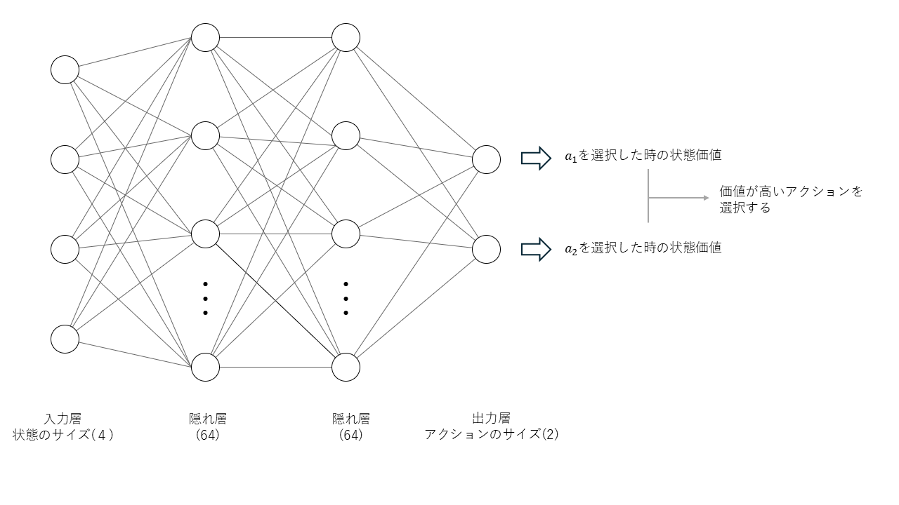
DNN Architecture
#In this case, we will use a DNN with two hidden layers.[6] The input layer comprises 4 units to accept the state, and the number of units in the output layer matches the number of actions. Each unit in the output layer represents the action value corresponding to that action, and the action with the highest value is chosen for execution.
Training the DNN
#Generally, training a neural network requires a dataset. However, in reinforcement learning, instead of using a pre-prepared dataset, the agent utilizes data generated through interactions with the environment. In a Q-network, the framework still involves defining a loss function and minimizing it just like with conventional neural networks. The loss function is defined to minimize the difference between the target value and the current value .
Here, is called the target, defined as:
- : The reward obtained when taking action
- : The action value when choosing the action with the highest value
Learning Process
#Let’s summarize the process described so far. The following steps are repeated until learning is complete:
- The agent obtains the initial state from the environment.
- Repeat the following until the end of learning:
- The agent selects an action from the current state (using the action value function).
- The state of the environment changes as a result of the agent executing the action.
- The environment returns a reward to the agent based on the action taken and the resulting state.
- The agent updates the action value function (Q-network) using the stored states, actions, and rewards.

Practical Implementation of Learning Using the DQN Algorithm
#We now tackle the CartPole task. The source code used in this article is uploaded in the repository below.
Class Structure
#As mentioned at the beginning, CartPole is a task included in the Gymnasium reinforcement learning library. Since the Env (environment) class is provided by Gymnasium, we only need to implement the other classes.
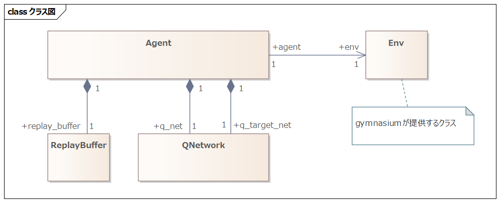
The ReplayBuffer class is used to store the history of states, actions, and rewards. The agent stores information in this class and retrieves data from it when updating the Q-network.
Execution and Results of Learning
#Running main.py will start the learning process.
from datetime import datetime

import gymnasium as gym
from agent import DQNAgent

# episode: number of episodes
episodes = 3000
# sync_interval: Interval to synchronize the Q-network
sync_interval = 20
env = gym.make("CartPole-v1", render_mode="human")
# env = gym.make("CartPole-v1")

agent = DQNAgent("cpu")
reward_history = []

for episode in range(episodes):
    observation, info = env.reset()
    done = False
    total_reward = 0.0
    print("episode: ", episode)

    while not done:
        # Provide the initial state and get an action
        action = agent.get_action(observation)

        # Step the environment to the next state
        next_obs, reward, terminated, truncated, info = env.step(action)

        agent.update(observation, action, reward, next_obs, terminated)
        observation = next_obs
        total_reward += reward
        env.render()
        if truncated or terminated:
            print("    done : total_reward: ", total_reward)
            print("    terminated: ", terminated, "truncated: ", truncated)
            done = True

    if episode % sync_interval == 0:
        agent.sync_qnet()


postfix = datetime.now().strftime("%Y%m%d_%H%M%S")
agent.save_model(postfix)
In the early stages of training (up to about 100 episodes), the agent quickly loses balance and the episode ends.
However, as training continues, the agent becomes better at maintaining balance. One way to verify whether training is progressing well is to look at a graph with the episode number on the x-axis and the cumulative reward on the y-axis. As training progresses, the cumulative reward should increase, resulting in an upward trending graph. Below is a sample graph from training over 3000 episodes.
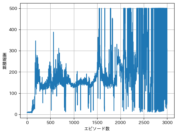
It can be seen that only after about 1500 episodes does the agent occasionally reach 500 steps, yet there are still episodes that end after just a few dozen steps. In the current method, the -greedy approach selects suboptimal actions with a certain probability, which can result in early failures even as training advances. To mitigate this effect, we trained for 3000 episodes 20 times and averaged the results, as shown in the graph below.
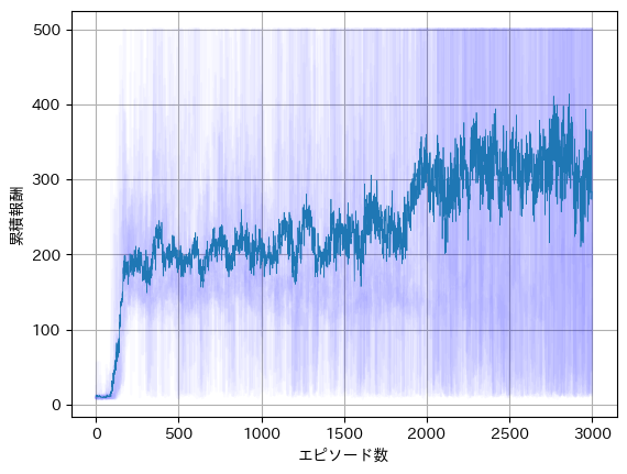
The solid line represents the average over 20 runs, while the individual graphs are shown faintly. Compared to the previous graph, an upward trend is clearly observed.
Saving and Utilizing the Trained Model
#Thus far, we have explained how the agent learns the CartPole task. Now, let’s discuss how to save and reuse the trained model. In this method, the neural network learns parameters that effectively approximate the action value function . By saving these parameters, you can reuse the trained model later.
The method for saving these trained parameters depends on the library. In PyTorch, which we used, the parameters can be saved to a file as follows:
def save_model(self, postfix: str):
    filename = f"q_net_{postfix}.pth"
    torch.save(self.qnet, filename)
During training, in order to experience a variety of states, actions were chosen at random with a certain probability. When deploying the model, it is changed so that it always selects the action with the highest Q-value.
before (with exploration)
def get_action(self, state: np.ndarray) -> int:
    if np.random.rand() < self.epsilon:
        # Choose action randomly (exploration)
        return np.random.choice(self.action_size)
    else:
        # Choose the action with the highest Q-value (exploitation)
        state_as_tensor = torch.tensor(state[np.newaxis, :], dtype=torch.float32)
        qs = self.qnet(state_as_tensor)
        return qs.argmax().item()
after (without exploration)
def get_action(self, state: np.ndarray) -> int:
    # Choose the action with the highest Q-value (exploitation)
    state_as_tensor = torch.tensor(state[np.newaxis, :], dtype=torch.float32)
    qs = self.qnet(state_as_tensor)
    return qs.argmax().item()
An agent that always selects the optimal action without exploration can survive for 500 consecutive steps.
In Conclusion
#In this article, we introduced the basics of reinforcement learning using the CartPole task as an example. In the approach presented here, a neural network is used to convert the state into its corresponding action value, though neural networks can also be used for the policy function or combined in various ways. Moreover, in recent years, methods utilizing LLMs or VLMs instead of the simple networks described here have emerged. The ability to combine different techniques according to the task at hand is one of the fascinating aspects of reinforcement learning.
References
#Reinforcement Learning:An Introduction
Gymnasium is a Python library that provides a simulation environment to support the development and research of reinforcement learning algorithms. ↩︎
If the rewards are fixed values, as in this case, the return can be regarded as the sum of a geometric series, which can be proven to converge. ↩︎
An example of stochastic state transitions is a car’s slip. When the action “move forward” is selected, whether the car’s position changes normally or slips and does not change can be considered probabilistic. ↩︎
This graph was created using the output of the DNN, which will be discussed later. ↩︎
Deep Q-Network. https://arxiv.org/abs/1312.5602 ↩︎
In DQN, the network architecture is not fixed to a specific shape. In this article, since the state is given as a 4-dimensional vector, we use a fully connected DNN. In the original paper, a CNN was used to extract features from game screens. ↩︎