Information

To reach a broader audience, this article has been translated from Japanese.
You can find the original version here.

This article is the Day 10 entry of the Mamezou Developer Site Advent Calendar 2025.

0. Introduction

In areas like robot control and image processing, you often need to solve optimization problems. Even within optimization, there are many types—linear programming, combinatorial optimization, and so on. Among these, the “least squares problem” is particularly common in practice. This problem seeks the parameter vector x that minimizes the following objective function F(x):
(Here, x is generally a vector.)

\min_{\boldsymbol{x}} F(\boldsymbol{x}) = \frac{1}{2} \sum_{i} \| r_i(\boldsymbol{x}) \|^2

Here, (r_i(\boldsymbol{x})) is called the residual, representing the difference between the observed data (measured value) (y_i) and the predicted value (theoretical value) (f_i(\boldsymbol{x})):

r_i(\boldsymbol{x}) = y_i - f_i(\boldsymbol{x})

In this article, we introduce Google’s solver “Ceres Solver”, which efficiently solves such nonlinear least squares problems.

1. Environment for This Article

This article targets Ubuntu 24.04. The author uses WSL2, but native Ubuntu works just as well.

Information

Although this article uses Ubuntu for the examples, Ceres Solver also works on Windows.
For details, see:
http://ceres-solver.org/installation.html#windows

2. Setting Up the Environment

These are the preparations needed to use CeresSolver. It’s a bit long, so thank you for your patience.

Installing Required Libraries

First, install the tools necessary to build Ceres Solver. Run each of the following lines one by one:

# apt update (you will be prompted for your password)
sudo apt update && sudo apt upgrade -y
# Build tools
sudo apt install build-essential
# Git
sudo apt install git
# CMake
sudo apt install cmake
# google-glog + gflags
sudo apt install libgoogle-glog-dev libgflags-dev
# Use ATLAS for BLAS & LAPACK
sudo apt install libatlas-base-dev
# Eigen3
sudo apt install libeigen3-dev
# SuiteSparse (optional)
sudo apt install libsuitesparse-dev

Creating the Workspace

Next, create a workspace. Here, we’ll make ceres_solver_ws in the home directory:

mkdir ~/ceres_solver_ws

Information

In a typical Linux environment, “~” represents your home directory, i.e. /home/${USER}/.

Cloning the CeresSolver Library

Once the workspace is ready, clone the CeresSolver source into an external directory. Use --recursive to fetch submodules:

cd ~/ceres_solver_ws
mkdir external
cd external
git clone --recursive https://github.com/ceres-solver/ceres-solver

Information

Alternatively, you can use:

git clone --recurse-submodules ${repo-url}

Building & Installing CeresSolver

Build CeresSolver with CMake:

cd ceres-solver
mkdir build
cmake -S . -B build
cmake --build build

If an error occurs when generating the build system

If you see:

CMake Error at CMakeLists.txt:33 (project):
  No CMAKE_CXX_COMPILER could be found.

install the build-essential package:

sudo apt install build-essential

Parallel Build Speedup

Building can take time. To speed it up with parallel jobs:

cmake --build build -- -j$(nproc)

nproc outputs the number of available CPU cores.

If you see 100% completion like this, the build succeeded:

[100%] Built target pose_graph_3d

Finally, install:

sudo cmake --install build
source ~/.bashrc

3. Solving a Simple Optimization Problem

Creating the CMakeLists.txt and Source File

Return to ~/ceres_solver_ws and create CMakeLists.txt:

cd ~/ceres_solver_ws
touch CMakeLists.txt

Put this in CMakeLists.txt:

# Specify the minimum CMake version
cmake_minimum_required(VERSION 3.14)

# Define the project name
project(ceres-solver-sample)

# Output executables to the build directory
set(CMAKE_RUNTIME_OUTPUT_DIRECTORY ${CMAKE_BINARY_DIR})

# Find Ceres
find_package(Ceres REQUIRED)

# Add subdirectory
add_subdirectory(src)

Then create src/CMakeLists.txt:

cd ~/ceres_solver_ws/src
touch CMakeLists.txt

Put this in src/CMakeLists.txt:

# simple-ols
add_executable(simple-ols simple-ols.cpp)
target_link_libraries(simple-ols absl::log_initialize Ceres::ceres)

Finally, create simple-ols.cpp:

cd ~/ceres_solver_ws/src
touch simple-ols.cpp

The structure is:

ceres_solver_ws/
├── CMakeLists.txt
└── src/
    ├── CMakeLists.txt
    └── simple-ols.cpp

Implementing the Optimization Calculation

In simple-ols.cpp, write:

simple-ols.cpp

#include <ceres/ceres.h>
#include <glog/logging.h>
#include <iostream>

using ceres::AutoDiffCostFunction;
using ceres::CostFunction;
using ceres::Problem;
using ceres::Solver;

/// @brief Residual struct
/// @remark The optimization target is defined in the () operator
struct CostFunctor {
    template <typename T>
    bool operator()(const T* const x, T* residual) const {
        // The optimization target expression in this case
        residual[0] = T(5.0) - x[0];
        return true;
    }
};

/// @brief Main function
int main(int argc, char** argv) {
    // Define the initial value
    double initial_x = 1.0;
    double x = initial_x;

    // Define the cost function
    CostFunction* cost_function =
        new AutoDiffCostFunction<CostFunctor, 1, 1>();

    // Define the optimization problem
    Problem problem;
    problem.AddResidualBlock(cost_function, nullptr, &x);
    problem.SetParameterLowerBound(&x, 0, 0.0);
    problem.SetParameterUpperBound(&x, 0, 10.0);

    // Define solver options
    Solver::Options options;
    options.linear_solver_type = ceres::DENSE_QR;
    options.minimizer_progress_to_stdout = true;
    options.max_num_iterations = 10;

    // Summary of results
    Solver::Summary summary;

    // Run the optimization
    Solve(options, &problem, &summary);

    // Output results (x is updated)
    std::cout << summary.BriefReport() << std::endl;
    std::cout << "x: " << initial_x << " -> " << x << std::endl;

    return 0;
}

Program Details

Cost Definition

/// @brief Residual struct
/// @remark The optimization target is defined in the () operator
struct CostFunctor {
    template <typename T>
    bool operator()(const T* const x, T* residual) const {
        // The optimization target expression in this case
        residual[0] = T(5.0) - x[0];
        return true;
    }
};

The calculation goes in operator().
The template type T is used during optimization (specifically ceres::Jet).
Cast built-in types to T when needed.

Defining the Cost Function

CostFunction* cost_function =
    new AutoDiffCostFunction<CostFunctor, 1, 1>();

Template arguments:

Cost struct type
Residual dimension
Parameter dimension

Defining the Optimization Problem

Problem problem;
problem.AddResidualBlock(cost_function, nullptr, &x);
problem.SetParameterLowerBound(&x, 0, 0.0);
problem.SetParameterUpperBound(&x, 0, 10.0);

You can specify a loss function in the second argument of AddResidualBlock. See
http://ceres-solver.org/nnls_tutorial.html#robust-curve-fitting.

Build and Run

cd ~/ceres_solver_ws
cmake -S . -B bin
cmake --build bin
./bin/simple-ols

You should see:

iter      cost      cost_change  |gradient|   |step|    tr_ratio  tr_radius  ls_iter  iter_time  total_time
   0  8.000000e+00    0.00e+00    4.00e+00   0.00e+00   0.00e+00  1.00e+04        0    1.35e-05    4.40e-05
   1  7.998400e-08    8.00e+00    4.00e-04   0.00e+00   1.00e+00  3.00e+04        1    8.09e-05    1.88e-04
   2  8.886518e-17    8.00e-08    1.33e-08   4.00e-04   1.00e+00  9.00e+04        1    3.24e-05    2.39e-04
Ceres Solver Report: Iterations: 3, Initial cost: 8.000000e+00, Final cost: 8.886518e-17, Termination: CONVERGENCE
x: 1 -> 5

Changing the Input Parameter Bounds

Change the upper bound from 10 to 3:

problem.SetParameterUpperBound(&x, 0, 3.0);  // changed from 10 to 3

Rebuild and run; you’ll get:

iter      cost      cost_change  |gradient|   |step|    tr_ratio  tr_radius  ls_iter  iter_time  total_time
   0  8.000000e+00    0.00e+00    2.00e+00   0.00e+00   0.00e+00  1.00e+04        0    1.21e-05    4.23e-05
   1  2.000000e+00    6.00e+00    0.00e+00   0.00e+00   7.50e-01  1.14e+04        1    6.80e-05    1.66e-04
Ceres Solver Report: Iterations: 2, Initial cost: 8.000000e+00, Final cost: 2.000000e+00, Termination: CONVERGENCE
x: 1 -> 3

4. Numerically Solving the Inverse Kinematics of a 4-DOF Planar Manipulator

In Chapter 3, we solved a scalar optimization problem. Now, we tackle a more complex nonlinear problem: the inverse kinematics of a 4-DOF planar manipulator.

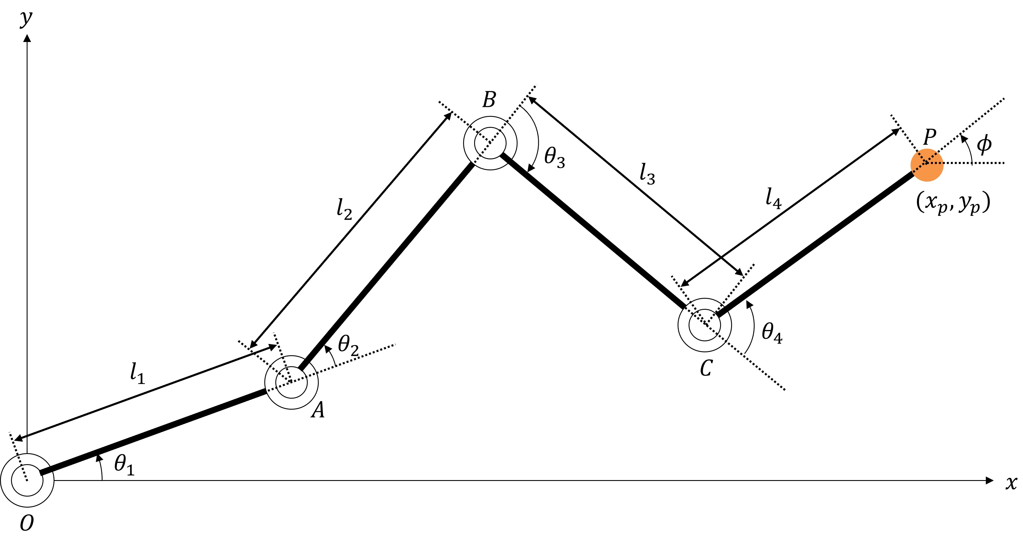
What is a 4-DOF Planar Manipulator?

Consider a planar manipulator with four joints as shown. We’ll implement its inverse kinematics. Parameters:

Link lengths: (L_i)
Joint angles: (\theta_i) (i=1..4), positive ccw
End effector position: ((x_p, y_p))
End effector orientation: (\phi)

Forward Kinematics Calculation

Define:
[
\boldsymbol{\theta} =
\begin{bmatrix}
\theta_1 \ \theta_2 \ \theta_3 \ \theta_4
\end{bmatrix}, \quad
\boldsymbol{p} =
\begin{bmatrix}
x_p \ y_p \ \phi
\end{bmatrix}.
]
Vectors:
[
\vec{OA} =
\begin{bmatrix}
L_1 \cos\theta_1 \ L_1 \sin\theta_1
\end{bmatrix},\quad
\vec{AB} =
\begin{bmatrix}
L_2 \cos(\theta_1+\theta_2) \ L_2 \sin(\theta_1+\theta_2)
\end{bmatrix},
]
[
\vec{BC} =
\begin{bmatrix}
L_3 \cos(\theta_1+\theta_2+\theta_3) \ L_3 \sin(\theta_1+\theta_2+\theta_3)
\end{bmatrix},\quad
\vec{CP} =
\begin{bmatrix}
L_4 \cos(\theta_1+\theta_2+\theta_3+\theta_4) \ L_4 \sin(\theta_1+\theta_2+\theta_3+\theta_4)
\end{bmatrix}.
]
Then:
[
\begin{bmatrix}
x_p \ y_p
\end{bmatrix}
= \vec{OA} + \vec{AB} + \vec{BC} + \vec{CP},\quad
\phi = \theta_1+\theta_2+\theta_3+\theta_4.
]
So:
[
\boldsymbol{p} = f(\boldsymbol{\theta}).
]

Inverse Kinematics Calculation

Inverse kinematics finds (\boldsymbol{\theta}) given (\boldsymbol{p}):
[
\boldsymbol{\theta} = f^{-1}(\boldsymbol{p}).
]
This is generally harder; we solve it numerically with CeresSolver.

Code Implementation

Creating Directories and CMakeLists.txt

cd ~/ceres_solver_ws/src
mkdir 4dof-ik
cd 4dof-ik
touch CMakeLists.txt

In src/CMakeLists.txt, add:

# simple-ols
add_executable(simple-ols simple-ols.cpp)
target_link_libraries(simple-ols absl::log_initialize Ceres::ceres)

# Register the 4dof-ik directory as a subdirectory
add_subdirectory(4dof-ik)

Defining Data Structures

cd ~/ceres_solver_ws/src/4dof-ik
touch Pose.hpp KinematicsParameters.hpp

Pose.hpp:

Pose.hpp

/// @brief Pose (position and orientation)
struct Pose {
    /// @brief X coordinate
    double x;
    /// @brief Y coordinate
    double y;
    /// @brief End effector orientation
    double phi;
    Pose(double x_, double y_, double phi_)
        : x(x_), y(y_), phi(phi_) {}
};

KinematicsParameters.hpp:

KinematicsParameters.hpp

/// @brief Kinematic parameters (link lengths)
struct KinematicParameters {
    /// @brief Link 1 length
    double L1;
    /// @brief Link 2 length
    double L2;
    /// @brief Link 3 length
    double L3;
    /// @brief Link 4 length
    double L4;
    /// @brief Constructor
    KinematicParameters(double l1, double l2, double l3, double l4)
        : L1(l1), L2(l2), L3(l3), L4(l4) {}
};

Implementing the Optimization Calculation

touch 4dof-ik.cpp

4dof-ik.cpp:

4dof-ik.cpp

#include <iostream>
#include <ceres/ceres.h>
#include <ceres/rotation.h>
#include <cmath>
#include "Pose.hpp"
#include "KinematicsParameters.hpp"

/// @brief Perform forward kinematics
template <typename T>
void compute_forward_kinematics(const KinematicParameters& kp,
                                const T* const theta,
                                T& x, T& y, T& phi) {
    x = T(kp.L1)*cos(theta[0])
      + T(kp.L2)*cos(theta[0]+theta[1])
      + T(kp.L3)*cos(theta[0]+theta[1]+theta[2])
      + T(kp.L4)*cos(theta[0]+theta[1]+theta[2]+theta[3]);
    y = T(kp.L1)*sin(theta[0])
      + T(kp.L2)*sin(theta[0]+theta[1])
      + T(kp.L3)*sin(theta[0]+theta[1]+theta[2])
      + T(kp.L4)*sin(theta[0]+theta[1]+theta[2]+theta[3]);
    phi = theta[0] + theta[1] + theta[2] + theta[3];
}

/// @brief Cost function for inverse kinematics
struct IKCostFunction {
    Pose target_pose;
    KinematicParameters kp;
    IKCostFunction(const Pose& pose, const KinematicParameters& param)
        : target_pose(pose), kp(param) {}
    template<typename T>
    bool operator()(const T* const theta, T* residuals) const {
        T x, y, phi;
        compute_forward_kinematics(kp, theta, x, y, phi);
        residuals[0] = T(target_pose.x) - x;    // X error
        residuals[1] = T(target_pose.y) - y;    // Y error
        residuals[2] = T(target_pose.phi) - phi; // Orientation error
        return true;
    }
};

int main(int argc, char** argv) {
    // Define kinematic parameters
    double l1 = 1.5, l2 = 1.5, l3 = 1.0, l4 = 1.0;
    // Define target pose
    double x_target = 3.2, y_target = 0.8, phi_target = -M_PI_4;
    // Initial joint angles
    double theta[4] = {0.0, 0.0, 0.0, 0.0};
    KinematicParameters kp(l1, l2, l3, l4);
    Pose target_pose{x_target, y_target, phi_target};

    // Define the optimization problem
    ceres::Problem problem;
    problem.AddResidualBlock(
        new ceres::AutoDiffCostFunction<IKCostFunction, 3, 4>(
            new IKCostFunction(target_pose, kp)),
        nullptr,
        theta);

    // Apply bounds (-π to π)
    for (int i = 0; i < 4; ++i) {
        problem.SetParameterLowerBound(theta, i, -M_PI);
        problem.SetParameterUpperBound(theta, i, M_PI);
    }

    // Solver options
    ceres::Solver::Options options;
    options.linear_solver_type = ceres::DENSE_QR;
    options.minimizer_progress_to_stdout = true;
    options.max_num_iterations = 100;
    options.function_tolerance = 1e-6;

    // Solve
    ceres::Solver::Summary summary;
    ceres::Solve(options, &problem, &summary);

    // Output results
    std::cout << summary.BriefReport() << std::endl;
    if (summary.termination_type == ceres::CONVERGENCE) {
        std::cout << "✅ IK Solution Found! (Final Cost: " << summary.final_cost << ")\n";
    } else {
        std::cout << "❌ IK Failed to Converge.\n";
    }
    // Output joint angles
    for (int i = 0; i < 4; ++i)
        std::cout << "theta[" << i << "] = " << theta[i] << std::endl;

    // Verify forward kinematics
    std::cout << "Check Forward Kinematics Calculation:" << std::endl;
    double x_result, y_result, phi_result;
    compute_forward_kinematics(kp, theta, x_result, y_result, phi_result);
    std::cout << "x   = " << x_result << std::endl;
    std::cout << "y   = " << y_result << std::endl;
    std::cout << "phi = " << phi_result << std::endl;

    return 0;
}

Adding to CMakeLists.txt

In 4dof-ik/CMakeLists.txt:

4dof-ik/CMakeLists.txt

# 4dof-ik
add_executable(4dof-ik 4dof-ik.cpp)
target_link_libraries(4dof-ik absl::log_initialize Ceres::ceres)

Build & Run

cd ~/ceres_solver_ws
cmake --build bin
./bin/4dof-ik

You should see:

Ceres Solver Report: Iterations: 7, Initial cost: 2.248425e+00, Final cost: 4.808292e-20, Termination: CONVERGENCE
✅ IK Solution Found! (Final Cost: 4.80829e-20)
theta[0] = -0.414376
theta[1] = 1.25568
theta[2] = 0.609086
theta[3] = -2.23579
Check Forward kinematics calculation:
x   = 3.2
y   = 0.8
phi = -0.785398

5. Conclusion

In this article, we introduced how to solve optimization problems using CeresSolver. Beyond the samples shown here, many examples are available on the official site:
http://ceres-solver.org/nnls_tutorial.html#non-linear-least-squares

The code from this article is also available at:
https://github.com/hayat0-ota/CeresSolver_tutorial